All Images
Introduction to Topological Data Analysis
Figure 1

Figure 2

Figure 3
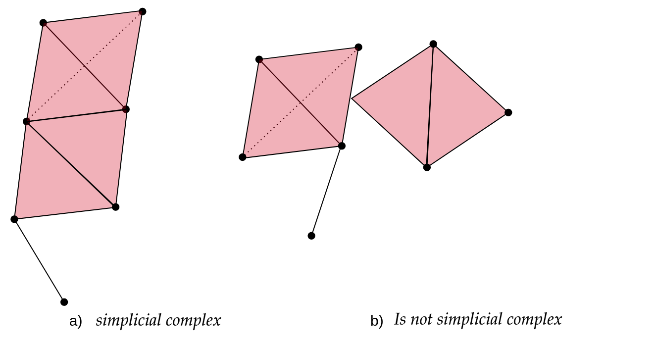
Figure 4
 > > In this figure, How many 0-simplices(vertices),
1-simplices(edges), and 2-simplices(triangles) does each one of the
simplicial complexes have? > > ## Solution > >
> > In this figure, How many 0-simplices(vertices),
1-simplices(edges), and 2-simplices(triangles) does each one of the
simplicial complexes have? > > ## Solution > >
> > | | Figure a | Figure b
|
> > |:———–:|:————:|:————:|
> > | \(0-simplex\) | 9 | 11
|
> > | \(1-simplex\) | 11 | 12
|
> > | \(2-simplex\) | 2 | 2
|
> > > {: .solution} {: .challenge}
Figure 5
Figure 6
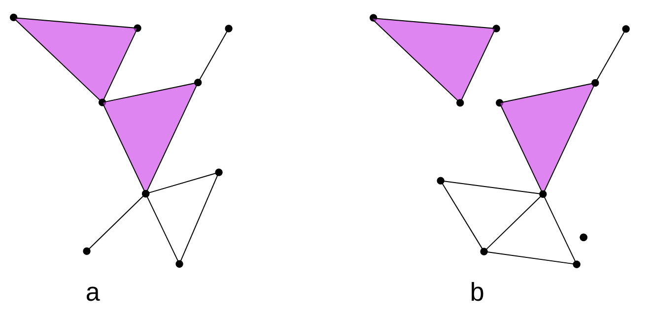
> > What are the \(\beta_0\)
and \(\beta_1\) of these simplicial
complexes in the image?. > > Hint: Remember that a painted
triangle (color rose in this case) represents a 2-simplex, while an
uncolored triangle represents a missing triangle that forms a 1-hole.
> > ## Solution
> >
> > | | Figure A | Figure B
|
> > |:———:|:————:|:————:|
> > | \(\beta_0\) | 1 | 3 |
> > | \(\beta_1\) | 1 | 2 |
> >
> {: .solution} {: .challenge}
Figure 7

Figure 8

Figure 9

Computational Tools for TDA
Figure 1

Figure 2

Figure 3
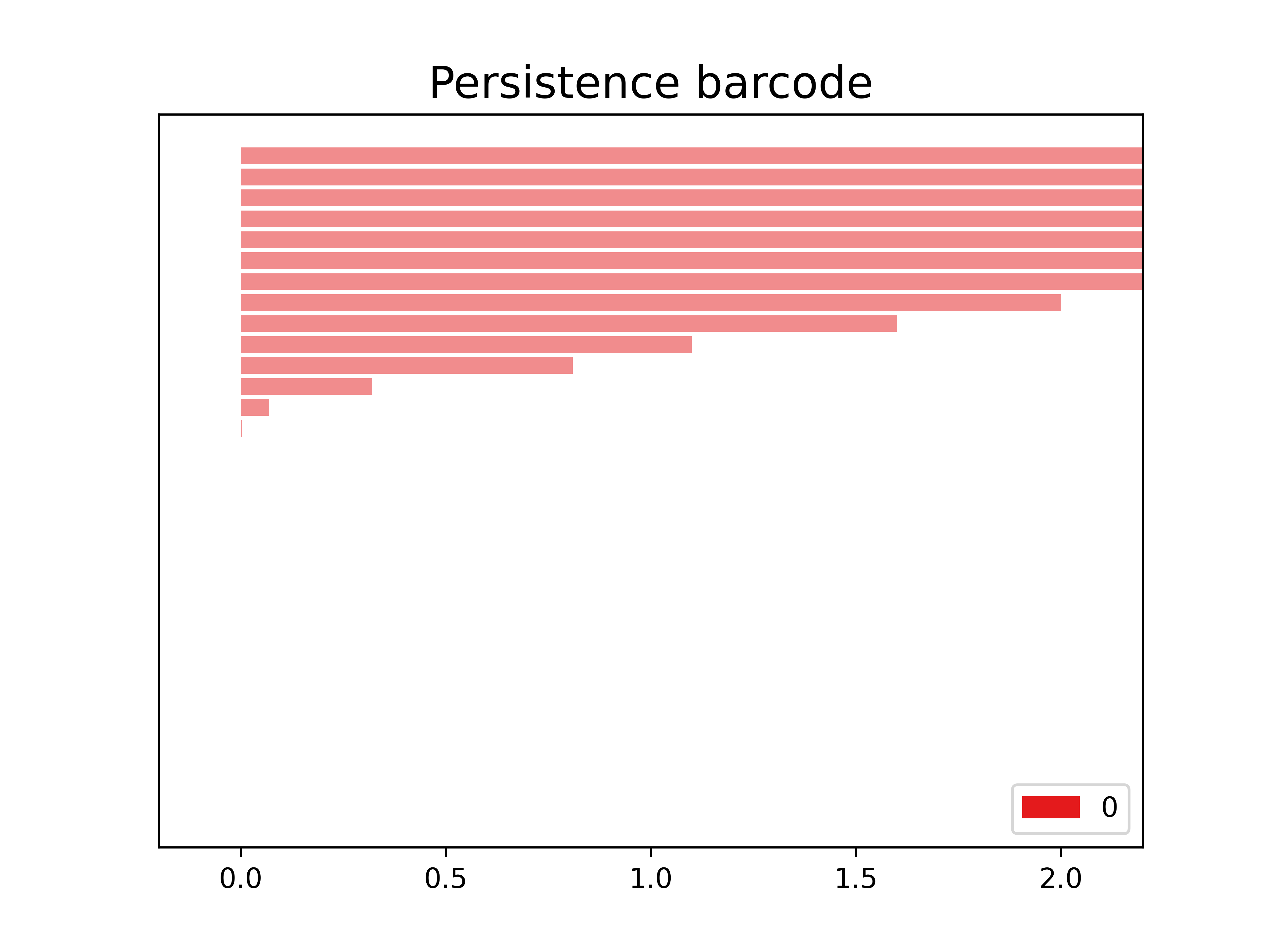
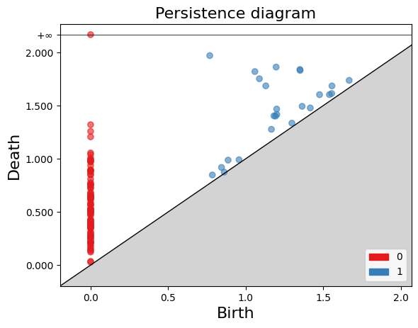
 > Perform persistent homology and plot the persistence diagram
and barcode. > > ## Solution
> Perform persistent homology and plot the persistence diagram
and barcode. > > ## Solution
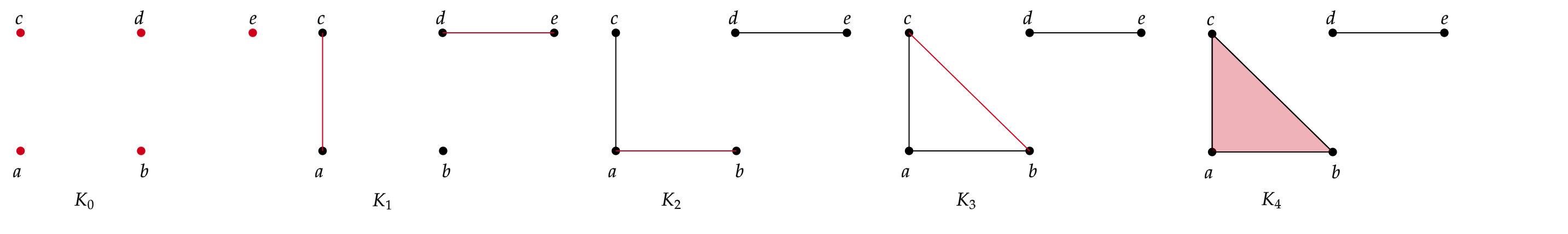
> > Step 1: Create a SimplexTree with
gd.SimplexTree(). > > ~ >> st =
gd.SimplexTree()
>> ~ >> {: .language-python}
>> Step 2: Insert vertices at time 0 using
st.insert() > > ~ >> #insert
0-simplex (the vertex), >> st.insert([0]) >> st.insert([1])
>> st.insert([2]) >> st.insert([3]) >> st.insert([4])
>> ~ >> {: .language-python}
>> Step 3: Insert the remaining simplices by setting the
filtration time using st.insert([0, 1], filtration=). >
> ~ >> #insert 1-simplex level filtration 1 >>
st.insert([0, 2], filtration=1) >> st.insert([3, 4], filtration=1)
>> #insert 1-simplex level filtration 2 >> st.insert([0, 1],
filtration=2) >> #insert 1-simplex level filtration 3 >>
st.insert([2, 1], filtration=3) >> #insert 1-simplex level
filtration 4 >> st.insert([2, 1,0], filtration=4) >>
~ >> {: .language-python}
>> Step 4: Perform persistent homology using
st.persistence(). > > ~ >># Compute
the persistence diagram >> persistence_diagram = st.persistence()
>> ~ >> {: .language-python}
>> Step 5: Plot the persistence diagram. > > ~
>># plot the persistence diagram >>
gd.plot_persistence_diagram(persistence_diagram,legend=True) >>
~ >> {: .language-python}
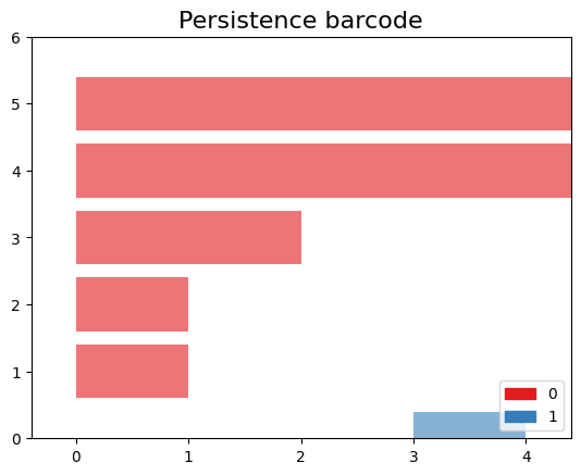
>> Step 6: Plot the barcode. > > ~ >>
gd.plot_persistence_barcode(persistence_diagram,legend=True) >>
~ >> {: .language-python}
>> Step 7: Get this output
>> >>
 >>
>>
> {: .solution} {: .challenge}
Figure 4
>>
>> Figure 5

Figure 6

Figure 7

Figure 8

Figure 9

Figure 10

Figure 11
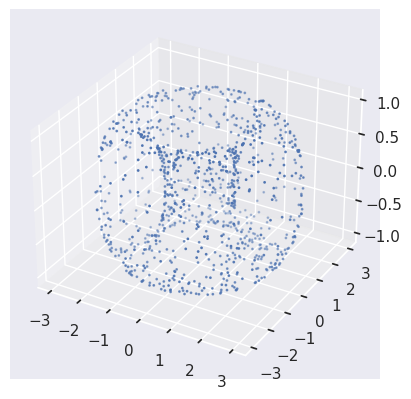
Figure 12
Detecting horizontal gene transfer
Figure 1
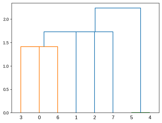
Figure 2
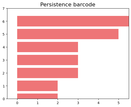
Figure 3
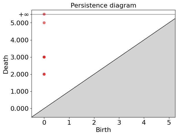
Figure 4
Figure 5
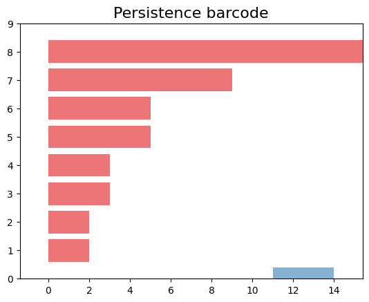
Figure 6
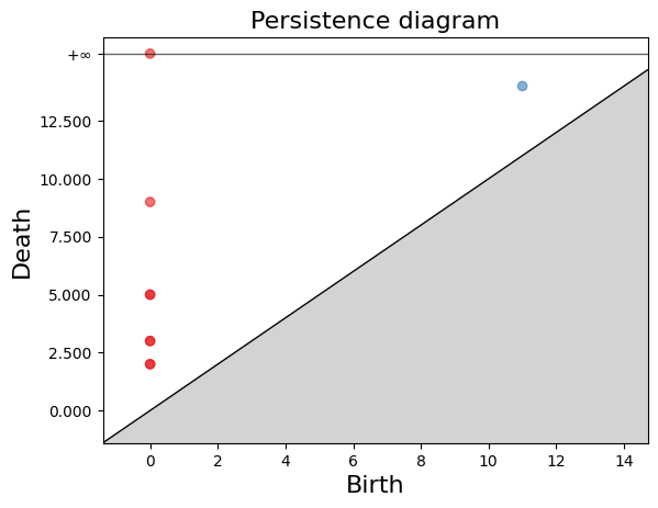
Figure 7
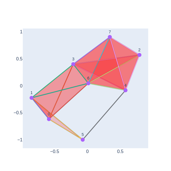
Figure 8

Figure 9
Persistence Simplices gives rise to Gene Families
Figure 1