All in One View
Content from Introduction to Genome Mining
Last updated on 2026-02-20 | Edit this page
Estimated time: 10 minutes
Overview
Questions
- What is Genome Mining?
Objectives
- Understand that Natural products are encoded in Biosynthetic Gene Clusters.
- Understand that Biosynthetic Gene Clusters can be identified in the genomic material.
- Discuss bioinformatic’s good practices with your colleagues.
What is Genome Mining?
In bioinformatics, genomic mining is defined as the computational analysis of nucleotide sequence data based on the comparison and recognition of conserved patterns. Under this definition, any computational method that involves searching for and predicting physiological or metabolic properties is considered part of genomic mining. The specific focus of genomic mining, when applied to natural products (NPs), is centered on the identification of biosynthetic gene clusters (BGCs) of NPs.
Natural products (NPs) are low molecular weight organic molecules that encompass a wide and diverse range of chemical entities with multiple biological functions. These molecules can be produced by bacteria, fungi, plants, and animals. Natural products (NPs) thus play various roles that can be analyzed from two main perspectives:
- Biological function: This refers to the role the molecule plays in the producing organism.
- Anthropocentric function: This focuses on the utility of NPs for humans, including their use in medicine, agriculture, and other areas.
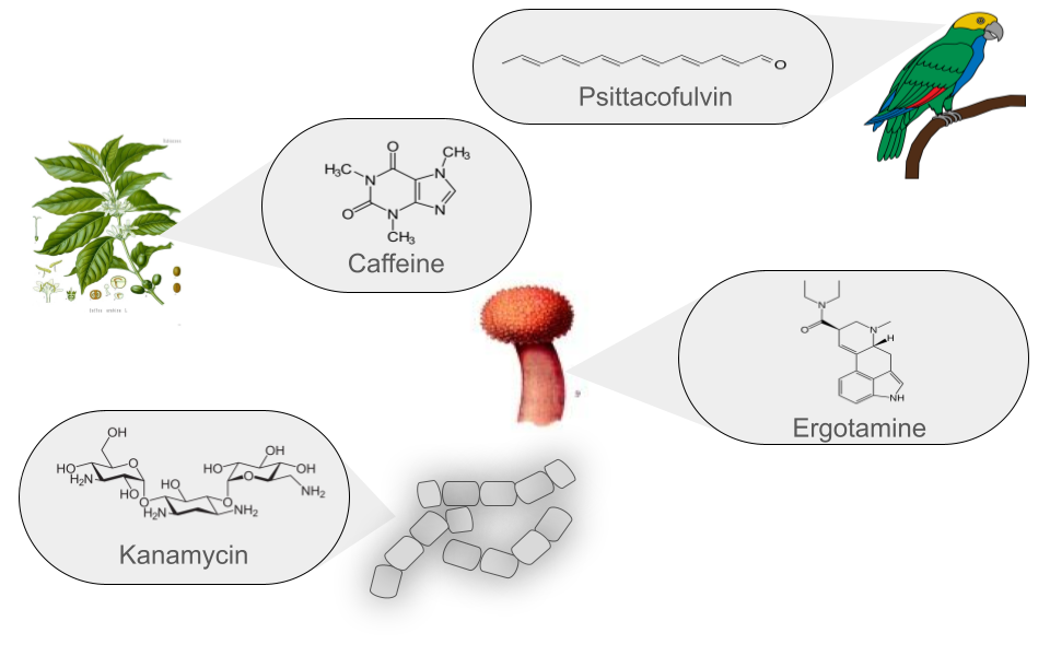
Currently, more than 126,000 NPs are known to originate from various sources and are classified into six main groups. These groups are defined based on their chemical structure, the enzymes involved in their synthesis, the precursors used, and the final modifications they undergo.
| Class | Description | Example |
|---|---|---|
| Polyketides (PKs) | Polyketides are organic molecules characterized by a repetitive chain of ketone (>C=O) and methylene (>CH2) groups. Their biosynthesis is similar to fatty acid synthesis, which is crucial to their diversity. These versatile molecules are found in bacteria, fungi, plants, and marine organisms. Notable examples include erythromycin, an antibiotic used to treat respiratory infections, and lovastatin, a lipid-lowering drug that reduces cholesterol. In summary, polyketides have a structure based on the repetition of ketone and methylene groups, with significant medical and pharmacological applications. | Erythromycin |
| Non-Ribosomal Peptides (NRPs) | NRPs are a family of natural products that differ from ribosomal peptides due to their non-linear synthesis. Their main structure is based on non-ribosomal modules, which include three key domains: Adenylation, acyl carrier, and condensation domain. Relevant examples include Daptomycin, an antibiotic widely used in various infections. Its NRP structure contributes to its antimicrobial activity. Cyclosporine is an immunosuppressant used in organ transplants. Its NRP structure is crucial to its function. In summary, NRPs feature a non-linear modular structure and play a significant role in medicine and chemical biology. | Daptomycin |
| Ribosomally synthesized and Post-translationally modified Peptides (RiPPs) | RiPPs are a diverse class of natural products of ribosomal origin. These peptides are produced in the ribosomes and then undergo enzymatic modifications after their synthesis. Historically, RiPPs were studied individually, but in 2013, uniform naming guidelines were established for these natural products. RiPPs include examples such as Microcin J25, an antibacterial RiPP produced by Escherichia coli, and Nisin, an antimicrobial RiPP produced by Lactococcus lactis. Their diversity and applications continue to be the subject of ongoing research. | Nisin |
| Saccharides | Saccharides produced in bacterial secondary metabolism are molecules synthesized by various mechanisms and then undergo subsequent enzymatic modifications based on the addition of carbohydrates. Two notable examples are Kanamycin, an aminoglycoside produced by Streptomyces kanamyceticus, used to treat bacterial infections, and Streptomycin, another aminoglycoside produced by Streptomyces griseus, which was one of the first antibiotics used to treat tuberculosis. Although their use has decreased due to bacterial resistance, they remain important in some cases. | Kanamycin |
| Terpenes | Traditionally, terpenes have been considered derivatives of 2-methyl-butadiene, better known as isoprene. Although they have been related to isoprene, terpenes do not directly derive from isoprene, as it has never been found as a natural product. The true precursor of terpenes is mevalonic acid, which comes from acetyl coenzyme A. Terpenes originate through the enzymatic polymerization of two or more isoprene units, assembled and modified in many different ways. Most terpenes have multicentric structures that differ not only in functional group but also in their basic carbon skeleton. These compounds are the main constituent of the essential oils of some plants and flowers, such as lemon and orange trees. They serve various functions in plants, such as being part of chlorophyll, carotenoid pigments, gibberellin and abscisic acid hormones, and increasing the fixation of proteins to cell membranes through isoprenylation. Additionally, terpenes are used in traditional medicine, aromatherapy, and as potential pharmacological agents. Two notable examples of terpenes are limonene, present in citrus peels and used in perfumery and cleaning products, and hopanoids, pentacyclic compounds similar to sterols, whose main function is to confer rigidity to the plasma membrane in prokaryotes. | Diplopterol |
| Alkaloids | Alkaloids are a class of natural, basic organic compounds that contain at least one nitrogen atom. They are mainly derived from amino acids and are characterized by their water solubility in acidic pH and solubility in organic solvents at alkaline pH. These compounds are found in various organisms, such as plants, fungi, and bacteria. Alkaloids have a wide range of pharmacological activities, such as Quinine, used against malaria, and Ephedrine, a bronchodilator. Additionally, some alkaloids, such as BE-54017, have an unusual structure, as it presents an indenotryptoline skeleton, rarely observed in other bis-indoles; however, its specific application is not well documented. | BE-54017 |
Genome mining aims to find BGCs
Natural products are encoded in Biosynthetic Gene Clusters (BGCs) in Bacteria. These BGCs are clusters of genes generally placed together in the same genome region. These include the genes encoding the biosynthetic enzymes and those related to the metabolite’s transport or resistance against antibacterial metabolites. Most BGCs are composed of several types of genes, so genome mining is based on the identification of these genes in a genome.
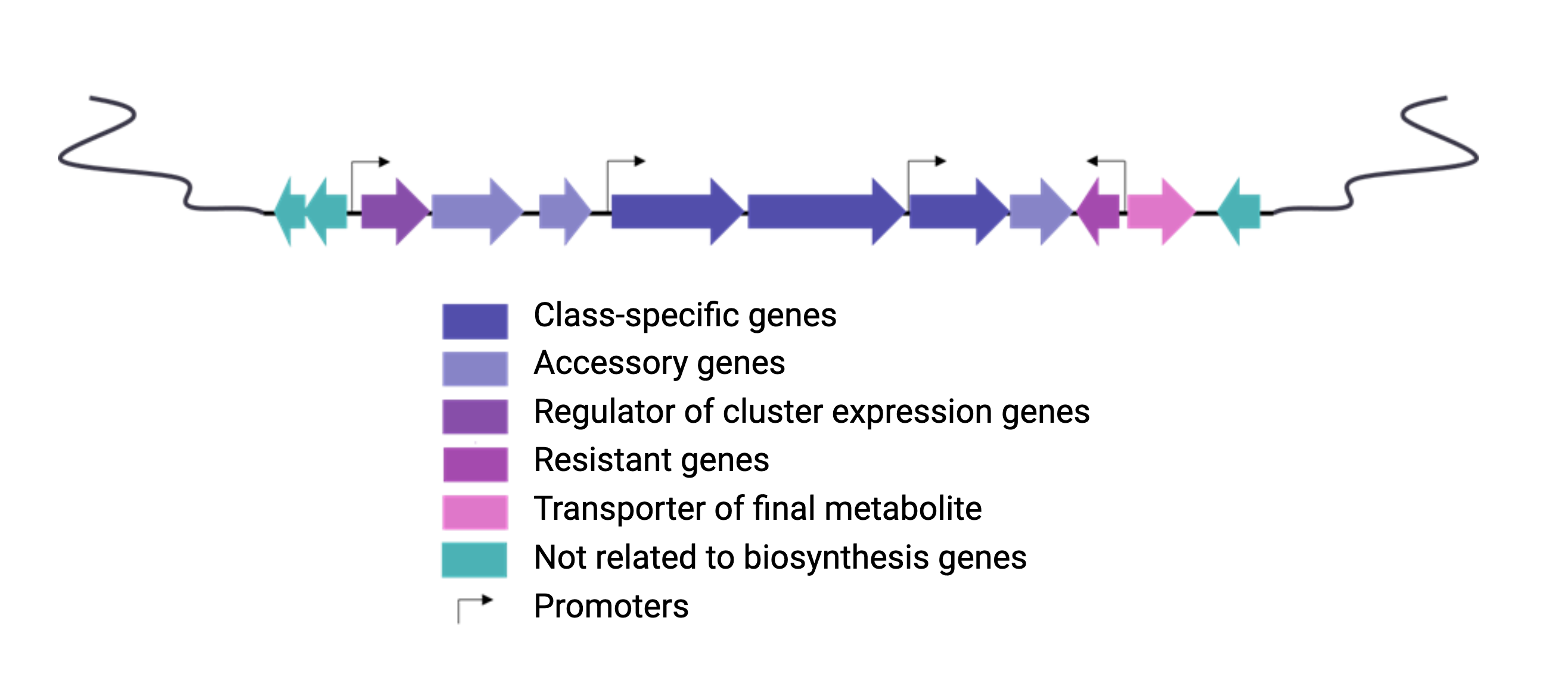
Each class of biosynthetic gene clusters (BGCs) is distinguished by the types of essential and accessory genes it contains. The most common classes of BGCs for natural products include polyketide synthases (PKSs), non-ribosomal peptide synthetases (NRPSs), ribosomally synthesized and post-translationally modified peptides (RiPPs), and terpenes. For example, non-ribosomal peptides (NRPs) are a class of metabolites characterized by the assembly of amino acid residues or their derivatives, with non-ribosomal peptide synthetases being the enzymes responsible for assembling these molecules. NRPSs are large enzymes organized into modules and domains, similar to other common classes of BGCs. Below, we show you an animation created by Michael W. Mullowney of the biosynthesis of a fictitious NP called “fakeomycin”, which is of the NRPS class with a cyclization domain.
Genome mining consists in analyzing genomes with specialized algorithms designed to find some BGCs. Chemists in the last century diligently characterized some of these clusters. We have extensive databases that contain information about which genes belong to which BGCs and some control sets of genes that do not. The use of genome mining methodologies facilitates the prioritization of BGCs for the search of novel metabolites. Since the era of next-generation sequencing, genomes have been explored as a source for discovering new BGCs.
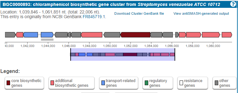
Chloramphenicol is a known antibiotic produced in a BGC
For example, let’s look into the BGC responsible for chloramphenicol biosynthesis. This is a BGC described for the first time in a Streptomyces venezuelae genome.
Exercise 1: Sort the Steps to Identify BGCs Similar to Clavulanic Acid
Below is a list of steps in disarray that are part of the process of identifying BGCs similar to clavulanic acid. Your task is to logically order them to establish a coherent methodology that allows the effective identification of such BGCs.
Disordered Steps:
Annotate the genes within the identified BGCs to predict their function.
Compare the identified BGCs against databases of known BGCs to find similarities to clavulanic acid.
Extract DNA from samples of interest, such as microorganism-rich soils or specific bacterial cultures.
Conduct phylogenetic analysis of the BGCs to explore their evolutionary relationship.
Use bioinformatics tools to assemble DNA sequences and detect potential BGCs.
Sequence the extracted DNA using next-generation sequencing (NGS) techniques.
- Extract DNA from samples of interest, such as microorganism-rich soils or specific bacterial cultures.
- Sequence the extracted DNA using next-generation sequencing (NGS) techniques.
- Use bioinformatics tools to assemble DNA sequences and detect potential BGCs.
- Annotate the genes within the identified BGCs to predict their function.
- Conduct phylogenetic analysis of the BGCs to explore their evolutionary relationship.
- Compare the identified BGCs against databases of known BGCs to find similarities to clavulanic acid.
Planning a genome mining project
Here we will provide tips and tricks to plan and execute a genome mining project. Firstly, choose a set of genomes from taxa. In this lesson we will be working with S. agalactiae genomes (Tettelin et al., 2005). Although this genus is not know for its potential as a Natural products producer, it is good enough to show different approaches to genome mining. Recently, metagenomes have been considered in genome mining studies. Here are some considerations that might be useful as a genome miner:
- Think about a research question before starting to analyze the data.
- Remember, raw metadata should remain intact during all genome mining processes. It could be a good idea to change its file permissions to read-only.
- Gather as much information as metadata of all the genomes you work with.
- All your intermediate steps should be considered temporal and may be removed without risk.
- Save your scripts using a version manager, GitHub for example.
- Share your data in public repositories.
- Give time to make your science repeatable and help your community.
Discussion 1: Describe your project
What are the advantages of documenting your work? Are there other things you can do to make your mining work more reproducible, like commenting on your scripts, etc.?
Documenting your work helps others (including your future self) understand what you have done and facilitates troubleshooting. To make your work more reproducible, you can detail the code logic by commenting on your scripts, use version control systems like Git, have backups of your scripts, share your data and code with others to facilitate feedback, and follow standardized workflows or protocols like those taught in this lesson. You can also name your files properly with a consistent format, structure your directories well, and back up your work regularly. Additionally, keeping a log (or “bitácora”) can serve as a tutorial for your future self, making it easier to understand your work later on.
Starting a genome mining project
Once you have chosen your set of genomes, you need to annotate the sequences. The process of genome annotation needs two steps. First, a gene calling approach (structural annotation), which looks for CDS or RNAs within the DNA sequences. Once these features have been detected, you need to assign a function for each CDS (functional annotation). This is usually done through comparison against protein databases. There are tens of bioinformatics tools to annotate genomes, but some of the most broadly used are; RAST (Aziz et al. 2008), and Prokka (Seeman, 2014). Here, we will start the genome mining lesson with S. agalactiae genomes already annotated by Prokka. You can download this data from this repository. The annotated genomes are written in GeneBank format (extension “.gbk”). To learn more about the basic annotation of genomes, see the lesson named “Pangenome Analysis in Prokaryotes: Annotating Genomic Data”. These files are also accessible in the… Insert introduction related to the access to the server??
References
- Aziz, R. K., Bartels, D., Best, A. A., DeJongh, M., Disz, T., Edwards, R. A., … & Zagnitko, O. (2008). The RAST Server: rapid annotations using subsystems technology. BMC genomics, 9(1), 1-15.
- Seemann, T. (2014). Prokka: rapid prokaryotic genome annotation. Bioinformatics, 30(14), 2068-2069.
- Tettelin, H., Masignani, V., Cieslewicz, M. J., Donati, C., Medini, D., Ward, N. L., … & Fraser, C. M. (2005). Genome analysis of multiple pathogenic isolates of Streptococcus agalactiae: implications for the microbial “pan-genome”. Proceedings of the National Academy of Sciences, 102(39), 13950-13955.
- Nett, Markus (2014). Kinghorn, A. D., ed. Genome Mining: Concept and Strategies for Natural Product Discovery. Springer International Publishing. pp. 199-245. ISBN 978-3-319-04900-7. doi:10.1007/978-3-319-04900-7\_4.
- Katz, Leonard; Baltz, Richard H. «Natural product discovery: past, present, and future». Journal of Industrial Microbiology and Biotechnology 43 (2-3): 155-176. ISSN 1476-5535. doi:10.1007/s10295-015-1723-5.
- Mejía Ponce, Paulina M.(2017). Análisis filogenético de familias de enzimas que utilizan tRNA, indicios para el descubrimiento de productos naturales ocultos en Actinobacteria. Tesis (M.C.)–Centro de Investigación y de Estudios Avanzados del I.P.N. Unidad Irapuato. Laboratorio Nacional de Genómica para la Biodiversidad. 2020-08-13T02:57:32Z.
- Natural products are encoded in Biosynthetic Gene Clusters (BGCs)
- Genome mining describes the exploitation of genomic information with specialized algorithms intended to discover and study BGCs
Content from Secondary metabolite biosynthetic gene cluster identification
Last updated on 2026-02-20 | Edit this page
Estimated time: 30 minutes
Overview
Questions
- How can I annotate known BGC?
- Which kind of analysis antiSMASH can perform?
- Which file extension accepts antiSMASH?
Objectives
- Understand antiSMASH applications.
- Perform a Minimal antiSMASH run analysis.
- Explore several Streptococcus genomes by identifying the BGCs presence and the types of secondary metabolites produced.
Introduction
Within microbial genomes, we can find some specific regions that take part in the biosynthesis of secondary metabolites, these sections are known as Biosynthetic Gene Clusters, which are relevant due to the possible applications that they may have, for example: antimicrobials, antitumors, cholesterol-lowering, immunosuppressants, antiprotozoal, antihelminth, antiviral and anti-aging activities.
What is a natural Product?
antiSMASH is a pipeline based on profile hidden Markov models that allow us to identify the gene clusters contained within the genome sequences that encode secondary metabolites of all known broad chemical classes.
antiSMASH input files
antiSMASH pipeline can work with three different file formats
GenBank, FASTA and EMBL. Both
GenBank and EMBL formats include genome
annotations, while a FASTA file just comprises the
nucleotides of each genomic contig.
Running antiSMASH
The command line usage of antiSMASH is detailed in the following repositories:
In summary, you will need to use your genome as the input. Then,
antiSMASH will create an output folder for each of your genomes. Within
this folder, you will find a single .gbk file for each of
the detected Biosynthetic Gene Clusters (we will use these files for
subsequent analyses) and a .html file, among others. By
opening the .html file, you can explore the antiSMASH
annotations.
You can run antiSMASH in two ways Minimal and Full-featured run, as follows:
| Run type | Command |
|---|---|
| Minimal run | antismash genome.gbk |
| Full-featured run | antismash –cb-general –cb-knownclusters –cb-subclusters –asf –pfam2go –smcog-trees genome.gbk |
Exercise 1: antiSMASH scope
If you run an Streptococcus agalactiae annotated genome using antiSMASH, what results do you expect?
The substances that a cluster produces
A prediction of the metabolites that the clusters can produce
A prediction of genes that belong to a biosynthetic cluster
- False. antiSMASH is not an algorithm devoted to substance
prediction.
- False. Although antiSMASH does have some information about
metabolites produced by similar clusters, this is not its main
purpose.
- True. antiSMASH compares domains and performs a prediction of the genes that belong to biosynthetic gene clusters.
Run your own antiSMASH analysis
First, activate the GenomeMining conda environment:
Second, run the antiSMASH command shown earlier in this lesson on the
data .gbk or .fasta files. The command can be
executed either in one single file, all the files contained within a
folder or in a specific list of files. Here we show how it can be
performed in these three different cases:
Running antiSMASH in a single file
Choose the annotated file ´agalactiae_A909_prokka.gbk´
BASH
$ mkdir -p ~/pan_workshop/results/antismash
$ cd ~/pan_workshop/results/antismash
$ antismash --genefinding-tool=none ~/pan_workshop/results/annotated/Streptococcus_agalactiae_A909_prokka/Streptococcus_agalactiae_A909_prokka.gbk
To see the antiSMASH generated outcomes do the following:
OUTPUT
.
├── CP000114.1.region001.gbk
├── CP000114.1.region002.gbk
├── css
├── images
├── index.html
├── js
├── regions.js
├── Streptococcus_agalactiae_A909.gbk
├── Streptococcus_agalactiae_A909.json
├── Streptococcus_agalactiae_A909.zip
└── svgVisualizing antiSMASH results
In order to see the results after an antiSMASH run, we need to access
to the index.html file. Where is this file located?
OUTPUT
~/pan_workshop/results/antismash/Streptococcus_agalactiae_A909_prokkaAs outcomes you should get a folder comprised mainly by the following files:
-
.gbkfiles For each Biosynthetic Gene cluster region found. -
.jsonfile To know the input file name, the antiSMASH used version and the regions data (id,sequence_data). -
index.htmlfile To visualize the outcomes from the analysis.
In order to access these results, we can use scp protocol to download the directory in your local computer.
If using scp , on your local machine, open a GIT bash
terminal in the destiny folder and execute the
following command:
BASH
$ scp -r user@bioinformatica.matmor.unam.mx:~/pan_workshop/results/antismash/S*A909.prokka/* ~/Downloads/.If using R-studio then in the left panel, choose the “more” option, and “export” your file to your local computer. Decompress the Streptococcus_agalactiae_A909.prokka.zip file.
Another way to download the data to your computer, you first compress the folder and download the compressed file from JupyterHub
BASH
$ cd ~/pan_workshop/results/antismash
$ zip -r Streptococcus_agalactiae_A909_prokka.zip Streptococcus_agalactiae_A909_prokka
$ ls
In the JupyterHub, navigate to the pan_workshop/results/antismash/ folder, select the file we just created, and press the download button at the top
Once in your local machine, in the directory,
Streptococcus_agalactiae_A909.prokka, open the index.html
file on your local web browser.
Understanding the output
The visualization of the results includes many different options. To understand all the possibilities, we suggest reading the following tutorial:
Briefly, in the “Overview” page ´.HTML´ you can find all the regions found within every analyzed record/contig (antiSMASH inputs), and summarized all this information in five main features:
- Region: The region number.
- Type: Type of the product detected by antiSMASH.
- From,To: The region’s location (nucleotides).
- Most similar known cluster: The closest compound from th MIBiG database.
- Similarity: Percentage of genes within the closest known compound that have significant BLAST hit (The last two columns containing comparisons to the MIBiG database will only be shown if antiSMASH was run with the KnownClusterBlast option ´–cc-mibig´).
antiSMASH web services
antiSMASH can also be used in an online server in the antiSMASH website: You will be asked to give your email. Then, the results will be sent to you and you will be allowed to donwload a folder with the annotations.
Exercises and discussion
Exercise 2: NCBI and antiSMASH webserver
Run antiSMASH web server over S. agalactiae A909. First, explore the NCBI assembly database to obtain the accession. Get the id of your results.
- Go to NCBI and search S. agalactiae A909.
- Choose the assembly database and copy the GenBank sequence ID at the bottom of the site.
- Go to antiSMASH
- Choose the accession from NCBI and paste
CP000114.1 - Run antiSMASH and paste into the collaborative document your results
id example
bacteria-cbd13a47-8095-495f-957c-dcf58c261529
Exercise 3: (*Optional exercise ) Run antiSMASH over thermophilus
Try Download and annotate S. thermophilus genomes strains LMD-9 (MiBiG), and strain CIRM-BIA 65 reference genome. With the following information, generate the script to run antiSMASH only on the S. thermophilus annotated genomes.
Guide to solve this problem First download genomes with genome-download. Remember to activate the conda environment!
Download the annotated genomes, and then the genbank files. 0.
ncbi-genome-download --formats genbank --genera "Streptococcus thermophilus" -S "LMD-9" -o thermophilus bacteria
ncbi-genome-download --formats fasta --genera "Streptococcus thermophilus" -S "CIRM-BIA 65" -n bacteria
Then, move the genomes to the directory
~/pan_workshop/results/annotated/S*.gbk
First, we need to start the for cycle:
for mygenome in ~/pan_workshop/results/annotated/S*.gbk
note that we are using the namemygenomeas the variable name in the for cycle.Then you need to use the reserved word
doto start the cycle.Then you have to call antiSMASH over your variable
mygenome. Remember the$before your variable to indicate to bash that now you are using the value of the variable.Finally, use the reserved word
doneto finish the cycle.
BASH
$ cd ~/pan_workshop/results/antismash
$ head Streptococcus_agalactiae_A909.prokka/CP000114.1.region001.gbk
$ grep LOCUS Streptococcus_agalactiae_A909.prokka/CP000114.1.region001.gbk
Locus contains the information of the characteristics of the sequence
In this case the size of the region is 42196 bp
Discussion 1: BGC classes in Streptococcus
What BGC classes does the genus Streptococcus have ?
In antiSMASH website output of A909 strain we see clusters of two classes, T3PKS and arylpolyene. Nevertheless, this is only one Streptococcus in order to infer all BGC classes in the genus we need to run antiSMASH in more genomes.
- antiSMASH is a bioinformatic tool capable of identifying, annotating and analysing secondary metabolite BGC
- antiSMASH can be used as a web-based tool or as stand-alone command-line tool
- The file extensions accepted by antiSMASH are GenBank, FASTA and EMBL
Content from Genome Mining Databases
Last updated on 2026-02-20 | Edit this page
Estimated time: 25 minutes
Overview
Questions
- Where can I find experimentally validated BGCs?
- Where is information about all predicted BGCs?
Objectives
- Use MIBiG database as a source of experimentally tested BGC.
- Explore antiSMASH database to learn about the distribution of predicted BGC.
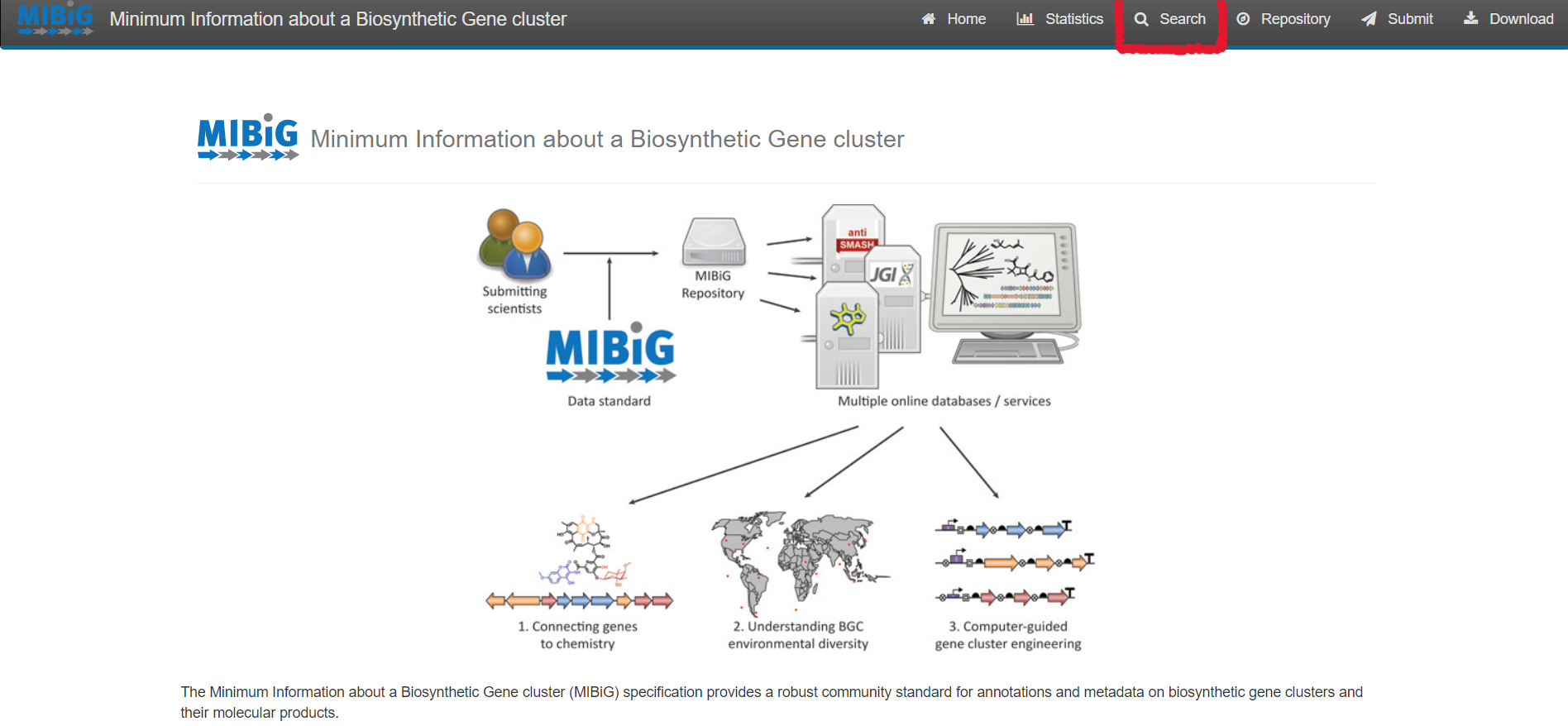
MIBiG Database
The Minimum Information about a Biosynthetic Gene cluster MIBiG is a database that facilitates consistent and systematic deposition and retrieval of data on biosynthetic gene clusters. MIBiG provides a robust community standard for annotations and metadata on biosynthetic gene clusters and their molecular products. It will empower next-generation research on the biosynthesis, chemistry and ecology of broad classes of societally relevant bioactive secondary metabolites, guided by robust experimental evidence and rich metadata components.
Browsing and Querying in the MIBiG database
Select “Search” on the upper right corner of the menu bar
For simple queries, such as Streptococcus agalactiae or searching for a specific strain you can use the “Simple search” function.
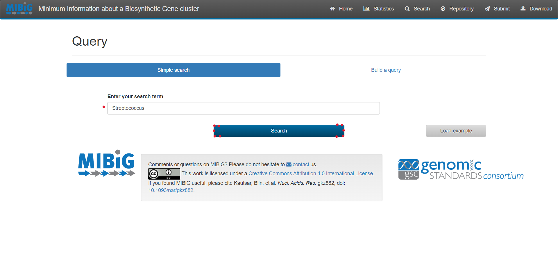
For complex queries, the database also provides a sophisticated query builder that allows querying on all antiSMASH annotations. To enable this function, click on “Build a query”
Results
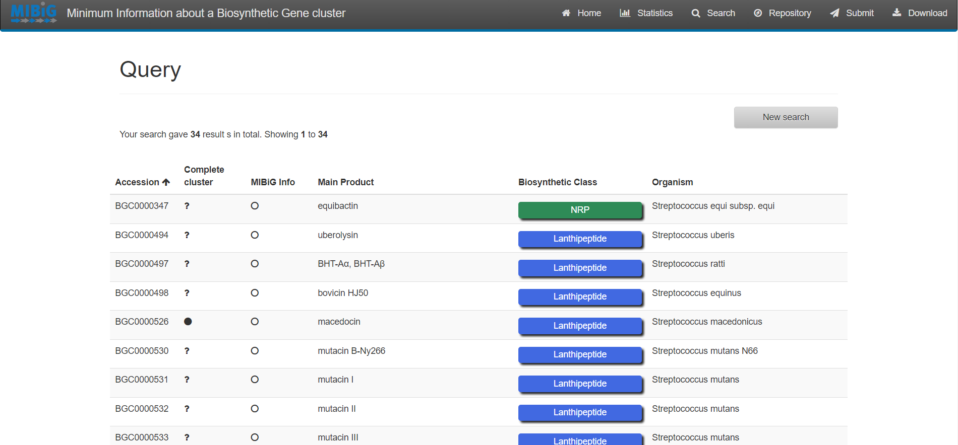
Exercise 1:
Enter to MIBiG and search BGCs from Streptococcus. Search the BGCs that produce the products Thermophilin 1277 and Streptolysin S. Based on the table on MIBiG, which of these organisms has the most complete annotation?
Streptococcus thermophilus produce Thermophilin 1277 while Streptococcus pyogenes M1 GAS produces Streptolysin S. According to MIBiG metadata Streptolysin S BGC is complete while Thermophilin 1277 is not. So Streptolysin S BGC is better annotated.
antiSMASH database
The antiSMASH database provides an easy to use, up-to-date collection of annotated BGC data. It allows to easily perform cross-genome analyses by offering complex queries on the datasets.
Browsing and Querying in the antiSMASH database
Select “Browse” on the top menu bar, alternatively you can select “Query” in the center
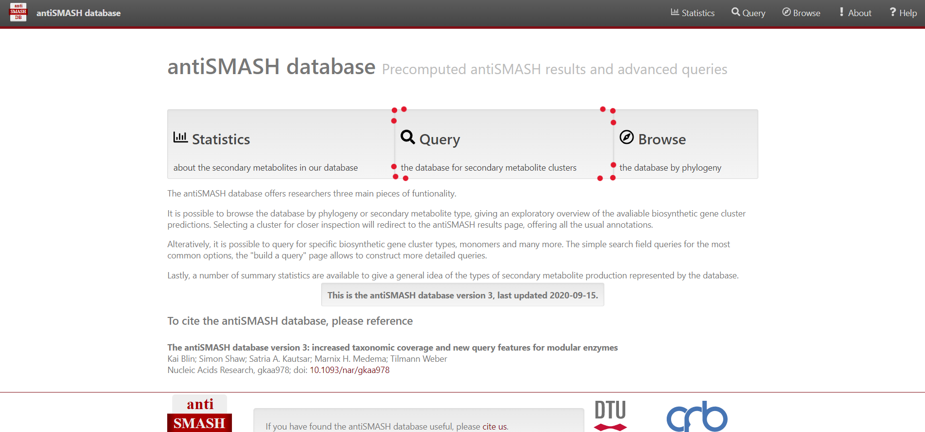
For simple queries, such as “Streptococcus” or searching for a specific strain you can use the “Simple search” function.
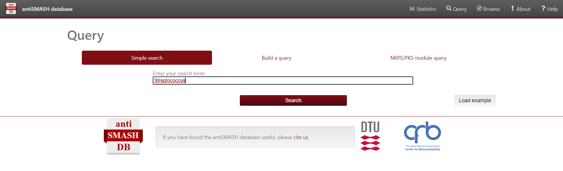
For complex queries, the database also provides a sophisticated query builder that allows querying on all antiSMASH annotations. To enable this function, click on “Build a query”
Results
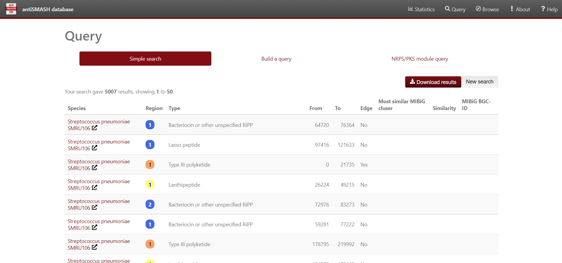
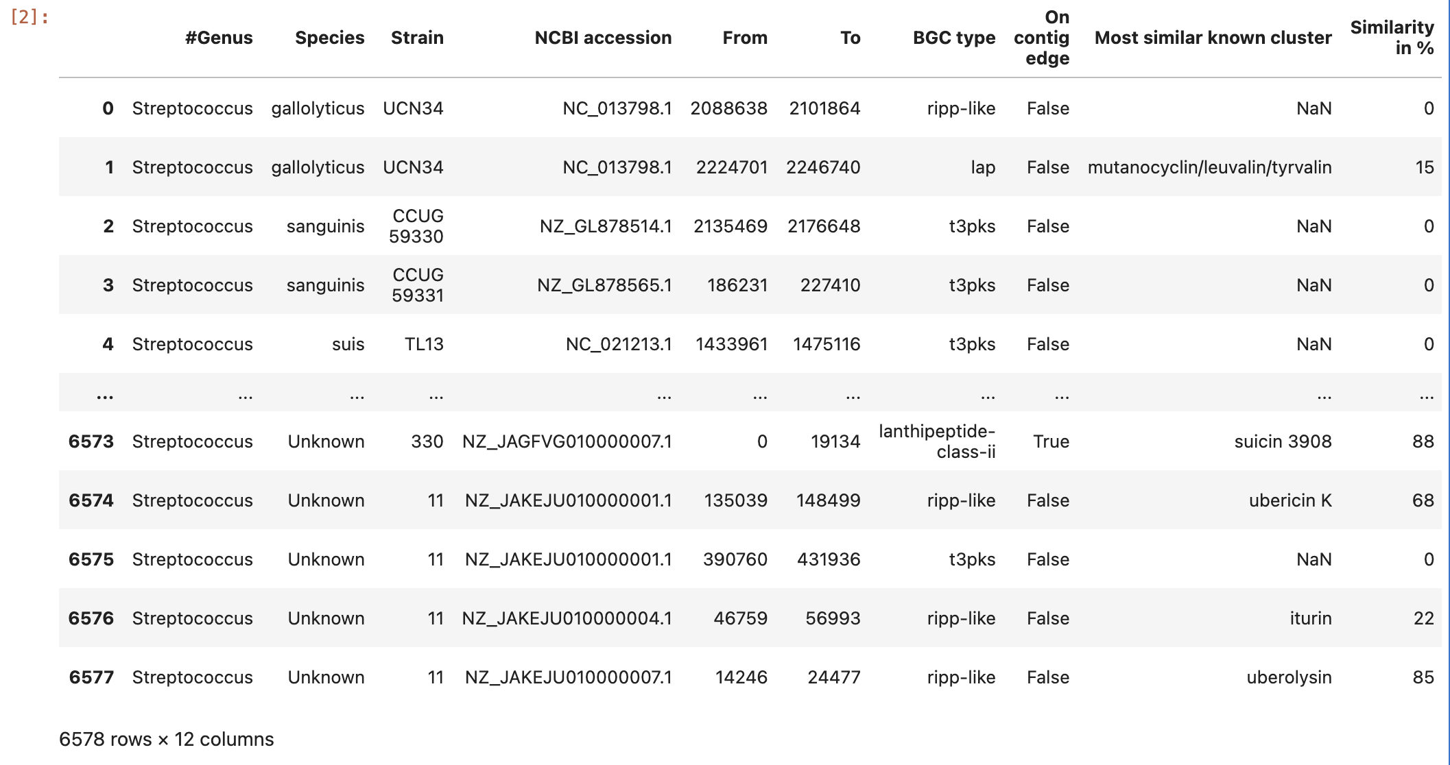
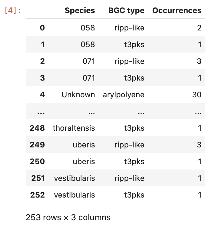
Use antiSMASH database to analyse the BGC contained in the Streptococcus genomes. We’ll use Python to visualize the data. First, import pandas, matplotlib.pyplot and seaborn libraries.
Secondly, store in a dataframe variable the content of the Streptococcus predicted BGC downloaded from antiSMASH-db.
PYTHON
data = pd.read_csv("https://raw.githubusercontent.com/AxelRamosGarcia/Genome-Mining/gh-pages/data/antismash_db.csv", sep="\t")
data
Now, group the data by the variables Species and BGC type:
And visualize the content of the ocurrences grouped by species column:
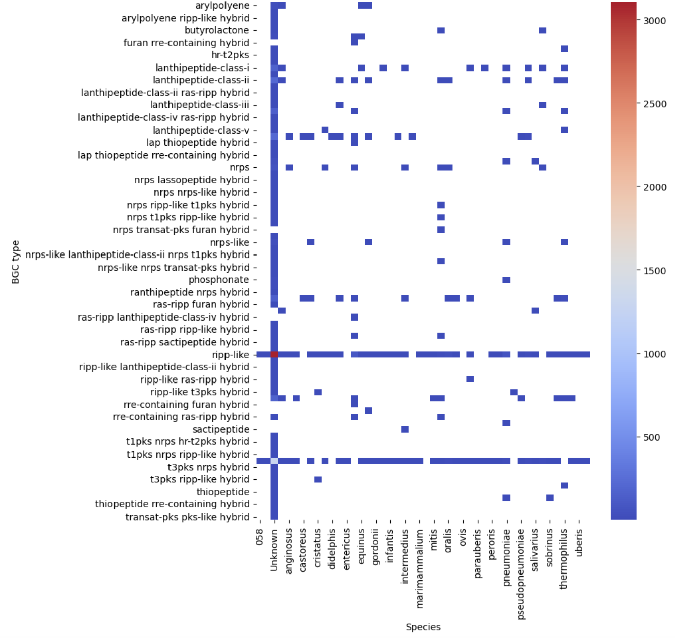
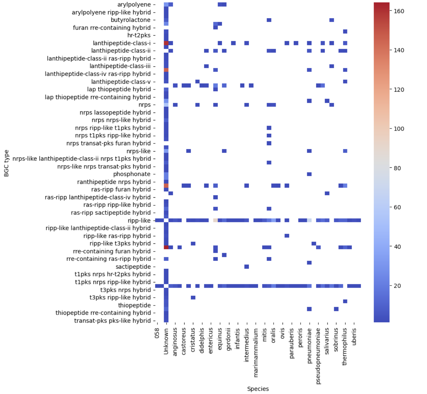
Let’s see our first visualization of the BGC content on a heatmap.
PYTHON
pivot = occurences.pivot(index="BGC type", columns="Species", values="Occurrences")
plt.figure(figsize=(8, 10))
sns.heatmap(pivot, cmap="coolwarm")
plt.show()
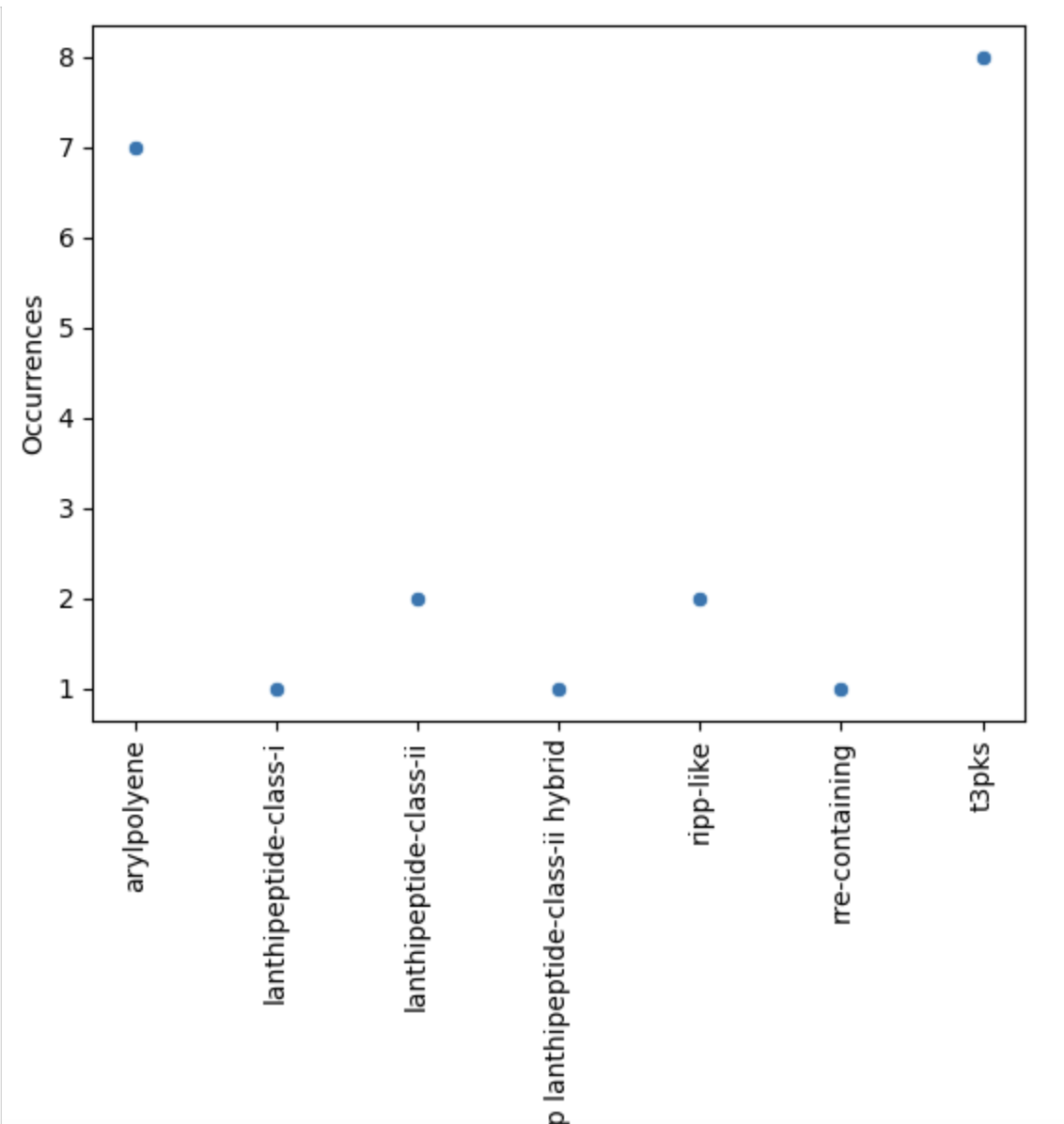
Now, let’s restrict ourselves to S. agalactiae.
PYTHON
agalactiae = occurences[occurences["Species"] == "agalactiae"]
sns.scatterplot(agalactiae, x="BGC type", y="Occurrences")
plt.xticks(rotation="vertical")
plt.show()
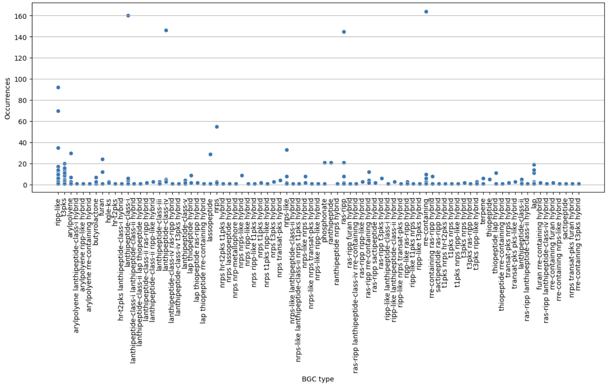
Finally, let’s restrict ourselves to BGC predicted less than 200 times.
PYTHON
filtered = occurences[occurences["Occurrences"] < 200]
plt.figure(figsize=(15, 5))
sns.scatterplot(filtered, x="BGC type", y="Occurrences")
plt.xticks(rotation="vertical")
plt.grid(axis="y")
plt.show()
PYTHON
filtered_pivot = filtered.pivot(index="BGC type", columns="Species", values="Occurrences")
plt.figure(figsize=(8, 10))
sns.heatmap(filtered_pivot, cmap="coolwarm")
plt.show()
- MIBiG provides BGCs that have been experimentally tested
- antiSMASH database comprises predicted BGCs of each organism
Content from BGC Similarity Networks
Last updated on 2026-02-20 | Edit this page
Estimated time: 45 minutes
Overview
Questions
- How can I measure similarity between BGCs?
Objectives
- Understand how BiG-SCAPE measures similarity between BGCs.
- Take an antiSMASH output to perform a BiG-SCAPE analysis.
- Interpret BiG-SCAPE similarity networks and GCF phylogenies.
Introduction
In the previous section, we learned how to study the BGCs encoded by each of the genomes of our analyses. In case you are interested in the study of a certain BGC or a certain strain, this may be enough. However, sometimes the aim is to compare the biosynthetic potential of tens or hundreds of genomes. To perform this kind of analysis, we will use BiG-SCAPE (Navarro-Muñoz et al., 2019), a workflow that compares all the BGCs detected by antiSMASH to find their relatedness. BiG-SCAPE will search for Pfam domains (Mistry et al., 2021) in the protein sequences of each BGC. Then, the Pfam domains will be linearized and compared, creating different similarity networks and scoring the similarity of each pair of clusters. Based on a cutoff value for this score, the diverse BGCs will be classified on Gene Cluster Families (GCFs) to facilitate their study. A single GCF is supposed to encompass BGCs that produce chemically related metabolites (molecular families). Lower cutoffs would create families of BGCs that produce identical compounds, while higher cutoffs would create families of more loosely related compounds.
Preparing the input
In each of the antiSMASH output directories, we will find a single
.gbk file for each BGC, which includes “region” within its
filename. Thus, we will copy all these files to the new directory.
Move into the directory that has the antiSMASH results of each genome:
BASH
$ conda deactivate
$ conda activate /miniconda3/envs/bigscape/
$ cd ~/pan_workshop/results/antismash/
$ ls
Since we will put together in the same directory many files with
similar names, we want to make sure that nothing is left behind or
overwritten. For this, we will count all the gbk files of
all the genomes.
OUTPUT
16Since the names are somewhat cryptic, they could be repeated, so we
will rename the gbks in such a way that they include the
genome name.
Copy the following script to a file named
change-names.sh using nano:
BASH
# This script is to rename the antiSMASH gbks for them to include the species and strain names, taken from the directory name.
# The argument it requires is the name of the directory with the AntiSMASH output, which must NOT contain a slash at the end.

# Usage for one AntiSMASH output directory:
#     sh change-names.sh <folder>

# Usage for multiple AntiSMASH output directory:
#     for species in <output-directory-pattern*>
#    	 do
#    		 sh change-names.sh $species
#    	 done


ls -1 "$1"/*region*gbk | while read line # enlist the gbks of all regions in the directory and start a while loop
 do
    dir=$(echo $line | cut -d'/' -f1) # save the directory name in a variable
    file=$(echo $line | cut -d'/' -f2) # save the file name in a variable
	for directory in $dir # start a for loop
    	do
   		 cd $directory # enter the directory
      	newfile=$(echo $dir-$file) # make a new variable that fuses the directory name with the file name
			 	echo "Renaming" $file " to" $newfile # print a message showing the old and new file names
			 	mv $file $newfile # rename
			 	cd .. # return to main directory before it begins again
		 done
 done
Run the script for all the directory:
Now make a directory for all your BiG-SCAPE analyses and inside it
make a directory that contains all of the gbks of all of
your genomes. This one will be the input for BiG-SCAPE. (For convenience
bigscape/ will be inside antismash/ while we
run BiG-SCAPE).
Now copy all the region gbksto this new directory, and
look at its content:
OUTPUT
Streptococcus_agalactiae_18RS21_prokka-AAJO01000016.1.region001.gbk
Streptococcus_agalactiae_18RS21_prokka-AAJO01000043.1.region001.gbk
Streptococcus_agalactiae_2603V_prokka-NC_004116.1.region001.gbk
Streptococcus_agalactiae_2603V_prokka-NC_004116.1.region002.gbk
Streptococcus_agalactiae_515_prokka-NZ_CP051004.1.region001.gbk
Streptococcus_agalactiae_515_prokka-NZ_CP051004.1.region002.gbk
Streptococcus_agalactiae_A909_prokka-NC_007432.1.region001.gbk
Streptococcus_agalactiae_A909_prokka-NC_007432.1.region002.gbk
Streptococcus_agalactiae_CJB111_prokka-NZ_AAJQ01000010.region001.gbk
Streptococcus_agalactiae_CJB111_prokka-NZ_AAJQ01000025.region001.gbk
Streptococcus_agalactiae_COH1_prokka-NZ_HG939456.1.region001.gbk
Streptococcus_agalactiae_COH1_prokka-NZ_HG939456.1.region002.gbk
Streptococcus_agalactiae_H36B_prokka-AAJS01000020.1.region001.gbk
Streptococcus_agalactiae_H36B_prokka-AAJS01000117.1.region001.gbk
Streptococcus_agalactiae_NEM316_prokka-NC_004368.1.region001.gbk
Streptococcus_agalactiae_NEM316_prokka-NC_004368.1.region002.gbk
Running BiG-SCAPE
BiG-SCAPE can be executed in different ways, depending on the
installation mode that you applied. You could call the program through
bigscape, run_bigscapeor
run_bigscape.py. Here, based on our installation (see Setup), we will use bigscape.
The options that we will use are described in the help page:
BASH
-i INPUTDIR, --inputdir INPUTDIR
                    	Input directory of gbk files, if left empty, all gbk
                    	files in current and lower directories will be used.

-o OUTPUTDIR, --outputdir OUTPUTDIR
                    	Output directory, this will contain all output data
                    	files.

--mix             	By default, BiG-SCAPE separates the analysis according
                   	to the BGC product (PKS Type I, NRPS, RiPPs, etc.) and
                   	will create network directories for each class. Toggle
                   	to include an analysis mixing all classes

--hybrids-off     	Toggle to also add BGCs with hybrid predicted products
                    	from the PKS/NRPS Hybrids and Others classes to each
                    	subclass (e.g. a 'terpene-nrps' BGC from Others would
                    	be added to the Terpene and NRPS classes)

--mode {global,glocal,auto}
                    	Alignment mode for each pair of gene clusters.
                    	'global': the whole list of domains of each BGC are
                    	compared; 'glocal': Longest Common Subcluster mode.
                    	Redefine the subset of the domains used to calculate
                    	distance by trying to find the longest slice of common
                    	domain content per gene in both BGCs, then expand each
                    	slice. 'auto': use glocal when at least one of the
                    	BGCs in each pair has the 'contig_edge' annotation
                    	from antiSMASH v4+, otherwise use global mode on that
                    	pair
We will use the option --mix to have an analysis of all
of the BGCs together besides the analyses of the BGCs separated by
class. The --hybrids-off option will prevent from having
the same BGC twice (in the case of hybrid BGCs that could belong to two
classes) in our results. And since none of the BGCs is on a contig edge,
we could use the global mode. However, frequently, when analyzing draft
genomes, this is not the case. Thus, the auto mode will be the most
appropriate, which will use the global mode to align domains except for
those cases in which the BGC is located near to a contig end, for which
the glocal mode is automatically selected. For this run we will use only
the default cutoff value (0.3).
Now we are ready to run BiG-SCAPE:
BASH
$ bigscape -i bigscape/bgcs_gbks/ -o bigscape/output_220124 --mix --hybrids-off --mode auto --pfam_dir /miniconda3/envs/bigscape/BiG-SCAPE-1.1.5/Output names
Most of the times you will need to re-run a software once you have explored the results; maybe you want to change parameters or add more samples. For this reason, you will need a flexible way to organize your project, including the names of the outputs. Usually, a good idea is to put the date in the name of the folder and keep track of the analyses you are running in your research notes.
Once the process is finished, you will find in your terminal screen
some basic results, such as the number of BGCs included in each type of
network. In the output folder you will find all the data.
Since BiG-SCAPE does not produce a file with the run information, it is
useful to copy the text printed on the screen to a file. Use
nano to paste all the text that BiG-SCAPE generated in a
file named bigscape.log inside the folder
output_100722/logs/.
Take a look at the BiG-SCAPE outputs:
OUTPUT
cache/ html_content/ index.html* logs/ network_files/ SVG/To keep ordered your directories, move your bigscape/
directory to results/:
And move the file change-names to folder
scripts/ in the pan_workshop/directory to save
our little script:
Viewing the results
An easy way to prospect your results is by opening the
index.html file with a browser (Firefox, Chrome, Safari,
etc.). In order to do this, you need to go to your local machine and
locate in the folder where you want to store your BiG-SCAPE results. Now
we compress the folder output_100622/ and download it to
your local machine.
In the JupyterHub we navigate to the folders and go to
/pan_workshop/results/bigscape and select the one we just
created output_220124.zip and download it.
On your local computer we unzip the files and open
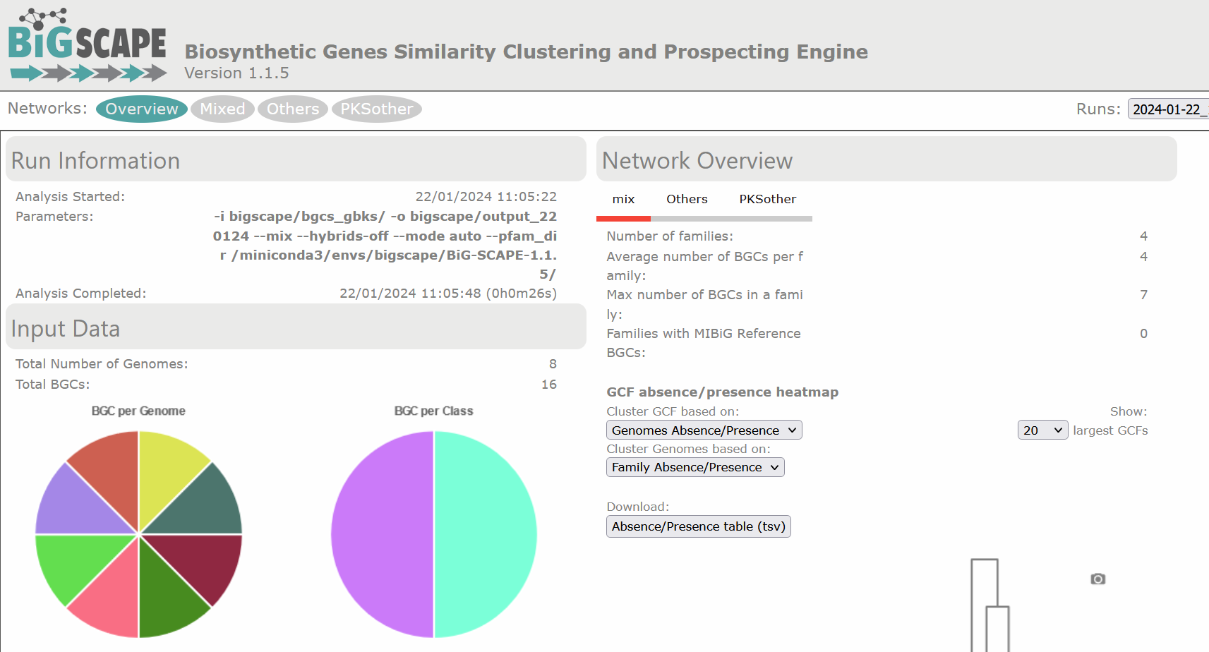
output_220124/index.html with a browser:
BASH
$ firefox output_100622/index.html # If you have Firefox available, otherwise open it using the GUI.There are diverse sections in the visualization. The following image shows the overview page. At the left there is the run information and there are pie chart representations of the number of BGCs per genome and per class. At the right there is the Network Overview for each of the BGC classes found and the mix category. They show the Number of Families, Average number of BGCs per family, Max number of BGCs in a family and the Families with MIBiG Reference BGCs. You can click on the name of the class to see its Network Overview.
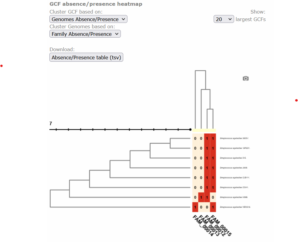
Below, there is a clustered heatmap of the presence/absence of the GCFs in each genome for each class. You can customize this heatmap and select the clustering methods, or the number of GCFs represented.
Clicking any of the class names of the upper left bar displays a similarity network of BGCs. It may take some time to load the network. A single network is represented for each GCF of each Gene Cluster Clan (GCC), which may comprise several GCFs. Each dot represents a BGC. These dots with bold circles are already described BGCs that have been recruited from the MiBIG database (Kautsar et al., 2020) because of its similarity with some BGC of the analysis.
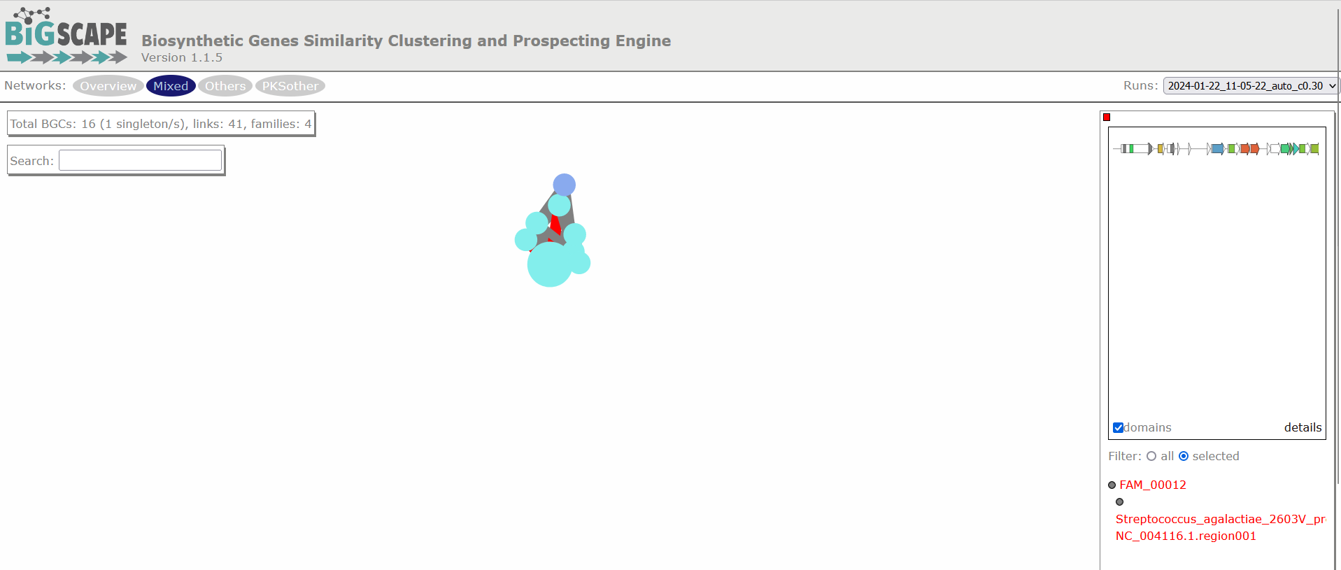
When you click on a BGC (dot), it appears its GCF at the right. You can click on the GCF name to see the phylogenetic distances among all the BGCs comprised by a single GCF. Within the tree there is an arrow diagram of the genes in the BGCs and the protein domains in the genes. These trees are useful to prioritize the search of secondary metabolites, for example, by focusing on the most divergent BGC clade or those that are distant to already described BGCs.
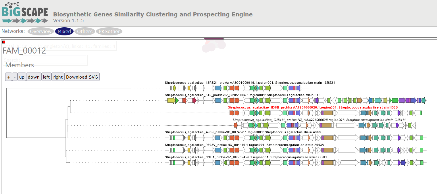
Discussion 1: Reading the GCF networks
What can you conclude about the diversity of BGCs between S. agalactiae and S. thermophilus? Are they equally diverse? Do they share GCFs?
Digging deeper: Why do you think the strain S. agalactiae H36B has a BGC that is not part of the other GCF in the same class?
S. agalactiae and S. thermophilus seem to have no diversity in common because there is no GCF with members from both species. All strains of S.agalactiae seem to have a very similar set of BGCs. While S. thermophilus has several BGCs that are not related to any other BGC.
Digging deeper: The BGC of the class PKSother in S. agalactiae H3B6 has only 3 genes, which are also present in the BGCs of the other GCF in this class. It is possible that these genes are in a fragmented part of the assembled genome, but are actually part of a BGC that is similar to the other ones. And it is also possible that these 3 genes are present in the genome without being part of a bigger BGC.
Exercise 1: Using the text output
Use one of the commands from the following list to make a reduced
version of the Network_Annotations_full.tsv, it should only
contain the information of the type of product, the BGC class of each
BGC, and its name. And save it in a file.
grep cut ls cat
mv
Tip: The file is inside
network_files/.
Take a look at the content of the file:
OUTPUT
BGC    Accession ID    Description    Product Prediction    BiG-SCAPE class    Organism    Taxonomy
Streptococcus_agalactiae_18RS21-AAJO01000016.1.region001    AAJO01000016.1    Streptococcus agalactiae
18RS21    arylpolyene    Others    Streptococcus agalactiae 18RS21    Bacteria,Terrabacteria
group,Firmicutes,Bacilli,Lactobacillales,Streptococcaceae,Streptococcus,Streptococcus agalactiae
Streptococcus_agalactiae_18RS21-AAJO01000043.1.region001    AAJO01000043.1    Streptococcus agalactiae
18RS21    T3PKS    PKSother    Streptococcus agalactiae 18RS21    Bacteria,Terrabacteria
group,Firmicutes,Bacilli,Lactobacillales,Streptococcaceae,Streptococcus,Streptococcus agalactiae
This table is difficult to read because of the amount of information
it has. The first line has the names of the columns; BGC,
Product Prediction and BiG-SCAPE class are the
ones we are interested in. So we will extract those.
BASH
cut -f 1,4,5 network_files/2022-06-10_21-27-26_auto/Network_Annotations_Full.tsv > type_of_BGC.tsv
cat type_of_BGCs.tsv
OUTPUT
BGC    Product Prediction    BiG-SCAPE class
Streptococcus_agalactiae_18RS21-AAJO01000016.1.region001    arylpolyene    Others
Streptococcus_agalactiae_18RS21-AAJO01000043.1.region001    T3PKS    PKSother
Streptococcus_agalactiae_515-AAJP01000027.1.region001    arylpolyene    Others
Streptococcus_agalactiae_515-AAJP01000037.1.region001    T3PKS    PKSother
.
.
.
Cytoscape visualization of the results
You can also customize and re-renderize the similarity networks of your results with Cytoscape (https://cytoscape.org/). To do so, you will need some files included in the output directory of BiG-SCAPE. Both are located in the same folder. You can choose any folder included in the Network_files/(date)hybrids_auto/ directory, depending on your interest. The “Mix/” folder represents the complete network, including all the BGCs of the analysis. There, you will need the files “mix_c0.30.network” and “mix_clans_0.30_0.70.tsv”. When you upload the “.network” file, it is required that you select as “source” the first column and as “target” the second one. Then, you can upload the “.tsv” and just select the first column as “source”. Finally, you need to click on Tools -> merge -> Networks -> Union to combine both GCFs and singletons. Now you can change colors, labels, etc. according to your specific requirements.
References
Navarro-Muñoz, J.C., Selem-Mojica, N., Mullowney, M.W. et al. “A computational framework to explore large-scale biosynthetic diversity”. Nature Chemical Biology (2019).
Mistry, J., Chuguransky, S., Williams, L., Qureshi, M., Salazar, G. A., Sonnhammer, E. L., … & Bateman, A. (2021). Pfam: The protein families database in 2021. Nucleic Acids Research, 49(D1), D412-D419.
Kautsar, S. A., Blin, K., Shaw, S., Navarro-Muñoz, J. C., Terlouw, B. R., van der Hooft, J. J., … & Medema, M. H. (2020). MIBiG 2.0: a repository for biosynthetic gene clusters of known function. Nucleic acids research, 48(D1), D454-D458.
- BGC similarity is measured by BiG-SCAPE according to protein domain content, adjacency and sequence identity.
- The
gbksof the regions identified by antiSMASH are the input for BiG-SCAPE. - BiG-SCAPE delivers BGCs similarity networks with which it delimits Gene Cluster Families and creates a phylogeny of the BGCs in each GCF.
Content from Homologous BGC Clusterization
Last updated on 2026-02-20 | Edit this page
Estimated time: 50 minutes
Overview
Questions
- How can I identify Gene Cluster Families?
- How can I predict the production of similar metabolites
- How can I clusterize BGCs into groups that produce similar metabolites?
- How can I compare the metabolic capability of different bacterial lineages?
Objectives
- Understand the purpose of using
BiG-SLiCEandBiG-FAM - Learn the inputs required to run
BiG-SLiCEandBiG-FAM - Run an example with our Streptococcus data on both softwares
- Understand the obtained results
BiG-SLiCE and BiG-FAM a set of tools to compare the microbial metabolic diversity
Around the curriculum, we have been learning about the metabolic capability of bacteria lineages encoded in BGCs. Before we start this lesson, let’s remember that the products of these clusters are biomolecules that are (mostly) not essential for life. They take the role of “tools” that offer some ecological and physiological advantage to the bacterial lineage producing it.
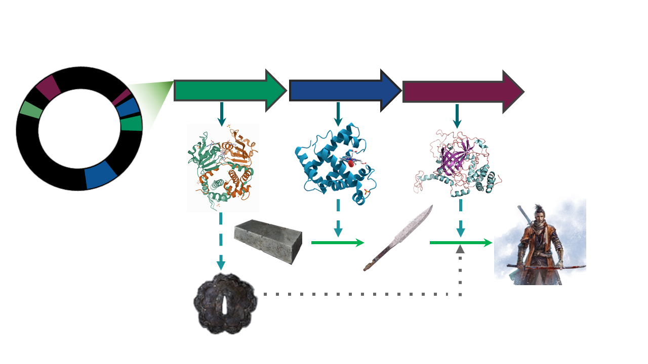
The presence/absence of a set of BGCs in a genome, can be associated to the ecological niches and (micro)environments which the lineage faces.
The counterpart of this can be taken as how biosynthetically diverse a bacterial lineage can be due to its environment.
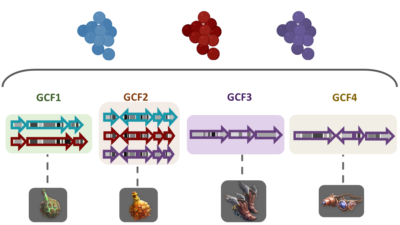
To answer some of this questions, we need a way to compare the metabolic capabilities of a set of diverse bacterial lineages. One way to do this is to compare the state (identity) of homologous BGCs. The homologous clusters that share a similar domain architecture and in consequence will produce a similar metabolite, are grouped into a bigger group that we call Gene Cluster Families (GCFs).
There are some programs capable of clustering BGCs in GCFs,
e.g.ClusterFinder and
DeepBGC.
BiG-SLICE is a software that has been designed
to do this work in less time, even when dealing with large datasets (1.2
million BGCs). This characteristic makes it a good tool to compare the
metabolic diversity of several bacterial lineages.
The input for BiG-SLiCE
Firstly, activate the conda environment, where BiG-SLiCE
has been installed as well as all the softwares required for its
usage:
You will have now a (GenomeMining) label at the
beginning of the prompt line.
If we seek for help using the --help flag of
bigslice, we can get a first glance at the input that we
need:
OUTPUT
usage: bigslice [-i <folder_path>] [--resume] [--complete] [--threshold T]
            	[--threshold_pct <N>] [--query <folder_path>]
            	[--query_name <name>] [--run_id <id>] [--n_ranks N_RANKS]
            	[-t <N>] [--hmmscan_chunk_size <N>] [--subpfam_chunk_size <N>]
            	[--extraction_chunk_size EXTRACTION_CHUNK_SIZE] [--scratch]
            	[-h] [--program_db_folder PROGRAM_DB_FOLDER] [--version]
            	<output_folder_path>

                        	_________
 ___	_____|\____|\____|\ \____	\
|   \  |   	} 	} 	}  ___)_ _/__
| >  | _--/--|/----|/----|/__/  __||  __|
|   < | ||  __/ (  (| | \___/  /__/|  _|
| >  || || |_ | _)  ) |_ | |\  \__ | |__
|____/|_| \___/|___/|___||_| \____||____| [ Version 1.1.0 ]

Biosynthetic Gene clusters - Super Linear Clustering Engine
(https://github.com/medema-group/bigslice)

positional arguments:
BiG-SLiCE is asking for a folder as the input. It is
important to highlight that the bones of this folder are the BGCs from a
group of genomes that has been obtained by antiSMASH. In
its GitHub page,
we can search for an input folder template.
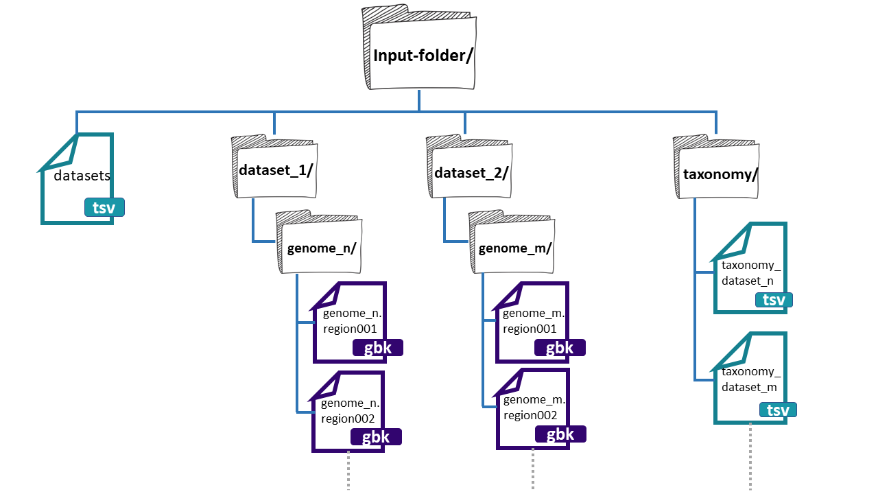
The folder needs three main components:
- datasets.tsv: This is a file that needs to have this exact name. This must be a tabular separated file where the information of each dataset (BGCs from a group of genomes) must be specified.

dataset_n: Each dataset will be composed by the BGCs of different genomes. We can give
BiG-SLiCEn groups of BGCs. The separation of the BGCs in different datasets is due to the different characteristics that the bacterial lineages can have. For example, if we have a set of bacterial populations that came from maize roots and other obtained from tomato roots, we can put them into dataset_1 and dataset_2 respectively.-
**taxonomy_n.tsv:**This is also a tabular separated file that will carry the taxonomic information of each of the genomes where the input BGCs were found and the path to reach these BGCs inside the input-folder:
- Genome folder name (ends with ‘/’)
- Kingdom / Domain name
- Class name
- Order name
- Family name
- Genus name
- Species name
- Organism / Strain name
Here, we have an example of the structure of the
input-folder:
Creating the input-folder
We will create a bigslice folder inside the
results directory.
Now that we know what input BiG-SLiCE requires, we will
do our input-folder step by step. First, let’s remember how many genomes
we have:
OUTPUT
agalactiae_18RS21/  agalactiae_A909/	agalactiae_COH1/
agalactiae_515/ 	agalactiae_CJB111/  agalactiae_H36B/
athermophilus_LMD-9/  athermophilus_LMG_18311/
We have six Streptococcus genomes from the original paper,
and two
public genomes. We will allocate their respective BGC .gbks
in two datasets, one for the genomes from Tettelin et
al. paper, and the other for the public ones.
BASH
$ mkdir input-folder
$ mkdir input-folder/dataset_1
$ mkdir input-folder/dataset_2
$ mkdir input-folder/taxonomy
$ tree
OUTPUT
.
└── input-folder
	├── dataset_1
	├── dataset_2
	└── taxonomy

4 directories, 0 files
Now we will create the folders for the BGCs of the dataset_1 genomes. We will take advantage of the strain name of our Streptococcus agalactiae lineages to create their folders:
BASH
$ for i in 18RS21 COH1 515 H36B A909 CJB111;
  do mkdir input-folder/dataset_1/Streptococcus_agalactiae_$i;
  done
$ tree -F
OUTPUT
.
└── input-folder/
	├── dataset_1/
	│   ├── Streptococcus_agalactiae_18RS21/
	│   ├── Streptococcus_agalactiae_515/
	│   ├── Streptococcus_agalactiae_A909/
	│   ├── Streptococcus_agalactiae_CJB111/
	│   ├── Streptococcus_agalactiae_COH1/
	│   └── Streptococcus_agalactiae_H36B/
	├── dataset_2/
	└── taxonomy/

10 directories, 0 files
We will do the same for the public genomes:
BASH
$ for i in LMD-9 LMG_18311;
  do mkdir input-folder/dataset_2/Streptococcus_thermophilus_$i;
  done
$ tree -F
BASH
.
└── input-folder/
	├── dataset_1/
	│   ├── Streptococcus_agalactiae_18RS21/
	│   ├── Streptococcus_agalactiae_515/
	│   ├── Streptococcus_agalactiae_A909/
	│   ├── Streptococcus_agalactiae_CJB111/
	│   ├── Streptococcus_agalactiae_COH1/
	│   └── Streptococcus_agalactiae_H36B/
	├── dataset_2/
	│   ├── Streptococcus_thermophilus_LMD-9/
	│   └── Streptococcus_thermophilus_LMG_18311/
	└── taxonomy/

12 directories, 0 files
Next, we will copy the BGCs .gbk files from the
dataset_1 genomes from each AntiSMASH output directory to
its respective folder .
BASH
$ ls input-folder/dataset_1/ | while read line;
  do cp ../antismash/output/$line/*region*.gbk input-folder/dataset_1/$line;
  done
$ tree -F
OUTPUT
.
└── input-folder/
	├── dataset_1/
	│   ├── Streptococcus_agalactiae_18RS21/
	│   │   ├── AAJO01000016.1.region001.gbk
	│   │   ├── AAJO01000043.1.region001.gbk
	│   │   └── AAJO01000226.1.region001.gbk
	│   ├── Streptococcus_agalactiae_515/
	│   │   ├── AAJP01000027.1.region001.gbk
	│   │   └── AAJP01000037.1.region001.gbk
	│   ├── Streptococcus_agalactiae_A909/
	│   │   ├── CP000114.1.region001.gbk
	│   │   └── CP000114.1.region002.gbk
	│   ├── Streptococcus_agalactiae_CJB111/
	│   │   ├── AAJQ01000010.1.region001.gbk
	│   │   └── AAJQ01000025.1.region001.gbk
	│   ├── Streptococcus_agalactiae_COH1/
	│   │   ├── AAJR01000002.1.region001.gbk
	│   │   └── AAJR01000044.1.region001.gbk
	│   └── Streptococcus_agalactiae_H36B/
	│   	├── AAJS01000020.1.region001.gbk
	│   	└── AAJS01000117.1.region001.gbk
	├── dataset_2/
	│   ├── Streptococcus_thermophilus_LMD-9/
	│   └── Streptococcus_thermophilus_LMG_18311/
	└── taxonomy/

12 directories, 13 files
Again, we will do the same for the BGCs .gbks of the
dataset_2:
BASH
$ ls input-folder/dataset_2/ | while read line;
  do cp ../antismash/output/$line/*region*.gbk input-folder/dataset_2/$line;
  done
$ tree -F
BASH
.
└── input-folder/
	├── dataset_1/
	│   ├── Streptococcus_agalactiae_18RS21/
	│   │   ├── AAJO01000016.1.region001.gbk
	│   │   ├── AAJO01000043.1.region001.gbk
	│   │   └── AAJO01000226.1.region001.gbk
	│   ├── Streptococcus_agalactiae_515/
	│   │   ├── AAJP01000027.1.region001.gbk
	│   │   └── AAJP01000037.1.region001.gbk
	│   ├── Streptococcus_agalactiae_A909/
	│   │   ├── CP000114.1.region001.gbk
	│   │   └── CP000114.1.region002.gbk
	│   ├── Streptococcus_agalactiae_CJB111/
	│   │   ├── AAJQ01000010.1.region001.gbk
	│   │   └── AAJQ01000025.1.region001.gbk
	│   ├── Streptococcus_agalactiae_COH1/
	│   │   ├── AAJR01000002.1.region001.gbk
	│   │   └── AAJR01000044.1.region001.gbk
	│   └── Streptococcus_agalactiae_H36B/
	│   	├── AAJS01000020.1.region001.gbk
	│   	└── AAJS01000117.1.region001.gbk
	├── dataset_2/
	│   ├── Streptococcus_thermophilus_LMD-9/
	│   │   ├── CP000419.1.region001.gbk
	│   │   ├── CP000419.1.region002.gbk
	│   │   ├── CP000419.1.region003.gbk
	│   │   ├── CP000419.1.region004.gbk
	│   │   └── CP000419.1.region005.gbk
	│   └── Streptococcus_thermophilus_LMG_18311/
	│   	├── NC_006448.1.region001.gbk
	│   	├── NC_006448.1.region002.gbk
	│   	├── NC_006448.1.region003.gbk
	│   	├── NC_006448.1.region004.gbk
	│   	├── NC_006448.1.region005.gbk
	│   	└── NC_006448.1.region006.gbk
	└── taxonomy/

12 directories, 24 filesExercise 1. Input-folder structure
As we have seen, the structure of the input folder for BiG-SLiCE is quite difficult to get. Imagine “Sekiro” wants to copy the directory structure to use it for future BiG-SLiCE inputs. Consider the following directory structure:
OUTPUT
  └── input_folder/
   	├── datasets.tsv
   	├── dataset_1/
   	|   ├── genome_1A/
   	|   |   ├── genome_1A.region001.gbk
   	|   |   └── genome_1A.region002.gbk
   	|   ├── genome_1B/
   	|   |   ├── genome_1B.region001.gbk
   	|   |   └── genome_1B.region002.gbk
   	├── dataset_2/
   	|   ├── genome_2A/
   	|   |   ├── genome_2A.region001.gbk
   	|   |   └── genome_2A.region002.gbk
   	|   ├── genome_2B/
   	|   |   ├── genome_2B.region001.gbk
   	|   |   └── genome_2B.region002.gbk
   	└── taxonomy/
       	├── taxonomy_dataset_1.tsv
       	└── taxonomy_dataset_2.tsv
Which would be the commands to copy the directory structure without
the files (just the folders)?
a)
BASH
$ mv -r input_folder input_folder_copy
$ rm input_folder_copy/dataset_1/genome_1A/* input_folder_copy/dataset_1/genome_1B/*
$ rm input_folder_copy/dataset_2/genome_2A/* input_folder_copy/dataset_2/genome_2B/*
$ rm input_folder_copy/taxonomy/*
BASH
$ cp -r input_folder input_folder_copy
$ rm input_folder_copy/dataset_1/genome_1A/* input_folder_copy/dataset_1/genome_1B/*
$ rm input_folder_copy/dataset_2/genome_2A/* input_folder_copy/dataset_2/genome_2B/*
$ rm input_folder_copy/taxonomy/*First we need to copy the whole directory to make an
input_folder_copy. After that we want to erase the files inside the
directories dataset_1/genome_1A, dataset_1/genome_1B,
dataset_2/genome_2A, dataset2/genome_2B and taxonomy/
c)
datasets.tsv file - The silmaril of BiG-SLiCE
The next step is to create the main file
datasets.tsv. First we put the first lines to this
file. In each of these .tsv files, we can put lines that
begin with #. This will not be read by the code, and it can
be of help to know which information is located in those files. We will
use the command echo with the -e flag that
will enable us to put tab separations between the text:
BASH
$ cd input-folder
$ echo -e "#Dataset name""\t""Path to folder""\t""Path to taxonomy""\t""Description" > datasets.tsv
$ more datasets.tsv
OUTPUT
#Dataset name Path to folder Path to taxonomy DescriptionWe will use echo One more time to put the
information of our two datasets. But this time, we will indicate bash
that we want to insert this new line in the existing
datasets.tsv with the >> option.
BASH
$ echo -e "dataset_1""\t""dataset_1/""\t""taxonomy/dataset_1_taxonomy.tsv""\t""Tetteling genomes" >> datasets.tsv
$ echo -e "dataset_2""\t""dataset_2/""\t""taxonomy/dataset_2_taxonomy.tsv""\t""Public genomes" >> datasets.tsv
$ more datasets.tsv
OUTPUT
#Dataset name   Path to folder  Path to taxonomy    	Description
dataset_1   	dataset_1/  	taxonomy/dataset_1_taxonomy.tsv Tetteling genomes
dataset_2   	dataset_2/  	taxonomy/dataset_2_taxonomy.tsv Public genomes
The main file of the input-folder is finished!
The taxonomy of the input-folder
We also need to specify the taxonomic assignation of each of the
input genomes BGC’s. We will build one dataset_taxonomy.tsv
file for each one of our datasets, i.e. two in total. Firstly,
create the header of each one of these files using
echo:
BASH
$ echo -e "#Genome folder""\t"Kingdom"\t"Phylum"\t"Class"\t"Order"\t"Family"\t"Genus"\t""Species Organism" > taxonomy/dataset_1_taxonomy.tsv
$ echo -e "#Genome folder""\t"Kingdom"\t"Phylum"\t"Class"\t"Order"\t"Family"\t"Genus"\t""Species Organism" > taxonomy/dataset_2_taxonomy.tsv

$ more taxonomy/dataset_1_taxonomy.tsv
OUTPUT
#Genome folder Kingdom Phylum Class Order Family Genus Species OrganismThere are several ways to obtain the taxonomic data. One of them is
searching for each lineage taxonomic identification on NCBI. There is
also a way to get this information from our .gbk files:
OUTPUT
LOCUS   	AAJO01000169.1      	2501 bp	DNA 	linear   UNK
DEFINITION  Streptococcus agalactiae 18RS21
ACCESSION   AAJO01000169.1
KEYWORDS	.
SOURCE  	Streptococcus agalactiae 18RS21.
  ORGANISM  Streptococcus agalactiae 18RS21
        	Bacteria; Terrabacteria group; Firmicutes; Bacilli;
        	Lactobacillales; Streptococcaceae; Streptococcus; Streptococcus
        	agalactiae.
FEATURES         	Location/Qualifiers
 	source      	1..2501
                 	/mol_type="genomic DNA"
                 	/db_xref="taxon:342613"
                 	/genome_md5=""
                 	/project="nselem35_342613"
                 	/genome_id="342613.37"
                 	/organism="Streptococcus agalactiae 18RS21"
 	CDS         	1..213
                 	/db_xref="SEED:fig|342613.37.peg.1973"
                 	/db_xref="GO:0003735"
We will use again echo to write this information into
our dataset_taxonomy.tsv. This is going to be a little long
because we have 8 genomes and we will need to write 8 echo
lines, but bear with us. We are almost there!
BASH
$ echo -e "Streptococcus_agalactiae_18RS21/""\t"Bacteria"\t"Firmicutes"\t"Bacilli"\t"Lactobacillales"\t"Streptococcaceae"\t"Streptococcus"\t""Streptococcus agalactiae 18RS21" >> taxonomy/dataset_1_taxonomy.tsv

$ echo -e "Streptococcus_agalactiae_515/""\t"Bacteria"\t"Firmicutes"\t"Bacilli"\t"Lactobacillales"\t"Streptococcaceae"\t"Streptococcus"\t""Streptococcus agalactiae 515" >> taxonomy/dataset_1_taxonomy.tsv

$ echo -e "Streptococcus_agalactiae_A909/""\t"Bacteria"\t"Firmicutes"\t"Bacilli"\t"Lactobacillales"\t"Streptococcaceae"\t"Streptococcus"\t""Streptococcus agalactiae A909" >> taxonomy/dataset_1_taxonomy.tsv

$ echo -e "Streptococcus_agalactiae_CJB111/""\t"Bacteria"\t"Firmicutes"\t"Bacilli"\t"Lactobacillales"\t"Streptococcaceae"\t"Streptococcus"\t""Streptococcus agalactiae CJB111" >> taxonomy/dataset_1_taxonomy.tsv

$ echo -e "Streptococcus_agalactiae_COH1/""\t"Bacteria"\t"Firmicutes"\t"Bacilli"\t"Lactobacillales"\t"Streptococcaceae"\t"Streptococcus"\t""Streptococcus agalactiae COH1" >> taxonomy/dataset_1_taxonomy.tsv

$ echo -e "Streptococcus_agalactiae_H36B/""\t"Bacteria"\t"Firmicutes"\t"Bacilli"\t"Lactobacillales"\t"Streptococcaceae"\t"Streptococcus"\t""Streptococcus agalactiae H36B" >> taxonomy/dataset_1_taxonomy.tsv

$ more taxonomy/dataset_1_taxonomy.tsv
OUTPUT
#Genome folder   Kingdom Phylum  Class   Order   Family  Genus   Species Organism
Streptococcus_agalactiae_18RS21/    	Bacteria    	Firmicutes  	Bacilli Lactobacillales Strept
ococcaceae  	Streptococcus   Streptococcus agalactiae 18RS21
Streptococcus_agalactiae_515/   Bacteria    	Firmicutes  	Bacilli Lactobacillales Streptococcace
ae  	Streptococcus   Streptococcus agalactiae 515
Streptococcus_agalactiae_A909/  Bacteria    	Firmicutes  	Bacilli Lactobacillales Streptococcace
ae  	Streptococcus   Streptococcus agalactiae A909
Streptococcus_agalactiae_CJB111/    	Bacteria    	Firmicutes  	Bacilli Lactobacillales Strept
ococcaceae  	Streptococcus   Streptococcus agalactiae CJB111
Streptococcus_agalactiae_COH1/  Bacteria    	Firmicutes  	Bacilli Lactobacillales Streptococcace
ae  	Streptococcus   Streptococcus agalactiae COH1
Streptococcus_agalactiae_H36B/  Bacteria    	Firmicutes  	Bacilli Lactobacillales Streptococcace
ae  	Streptococcus   Streptococcus agalactiae H36B
We will do the same for the dataset_2_taxonomy.tsv
file:
BASH
$ echo -e "Streptococcus_thermophilus_LMD-9/""\t"Bacteria"\t"Firmicutes"\t"Bacilli"\t"Lactobacillales"\t"Streptococcaceae"\t"Streptococcus"\t""Streptococcus thermophilus LMD-9" >> taxonomy/dataset_2_taxonomy.tsv

$ echo -e "Streptococcus_thermophilus_LMG_18311/""\t"Bacteria"\t"Firmicutes"\t"Bacilli"\t"Lactobacillales"\t"Streptococcaceae"\t"Streptococcus"\t""Streptococcus thermophilus LMG 18311" >> taxonomy/dataset_2_taxonomy.tsv

$ more taxonomy/dataset_2_taxonomy.tsv
OUTPUT
#Genome folder   Kingdom Phylum  Class   Order   Family  Genus   Species Organism
Streptococcus_thermophilus_LMD-9/   	Bacteria    	Firmicutes  	Bacilli Lactobacillales Strept
ococcaceae  	Streptococcus   Streptococcus thermophilus LMD-9
Streptococcus_thermophilus_LMG_18311/   Bacteria    	Firmicutes  	Bacilli Lactobacillales Strept
ococcaceae  	Streptococcus   Streptococcus thermophilus LMG 18311
Now, we have the organization of our input-folder
complete
OUTPUT
input-folder/
├── dataset_1/
│   ├── Streptococcus_agalactiae_18RS21/
│   │   ├── AAJO01000016.1.region001.gbk
│   │   ├── AAJO01000043.1.region001.gbk
│   │   └── AAJO01000226.1.region001.gbk
│   ├── Streptococcus_agalactiae_515/
│   │   ├── AAJP01000027.1.region001.gbk
│   │   └── AAJP01000037.1.region001.gbk
│   ├── Streptococcus_agalactiae_A909/
│   │   ├── CP000114.1.region001.gbk
│   │   └── CP000114.1.region002.gbk
│   ├── Streptococcus_agalactiae_CJB111/
│   │   ├── AAJQ01000010.1.region001.gbk
│   │   └── AAJQ01000025.1.region001.gbk
│   ├── Streptococcus_agalactiae_COH1/
│   │   ├── AAJR01000002.1.region001.gbk
│   │   └── AAJR01000044.1.region001.gbk
│   └── Streptococcus_agalactiae_H36B/
│   	├── AAJS01000020.1.region001.gbk
│   	└── AAJS01000117.1.region001.gbk
├── dataset_2/
│   ├── Streptococcus_thermophilus_LMD-9/
│   │   ├── CP000419.1.region001.gbk
│   │   ├── CP000419.1.region002.gbk
│   │   ├── CP000419.1.region003.gbk
│   │   ├── CP000419.1.region004.gbk
│   │   └── CP000419.1.region005.gbk
│   └── Streptococcus_thermophilus_LMG_18311/
│   	├── NC_006448.1.region001.gbk
│   	├── NC_006448.1.region002.gbk
│   	├── NC_006448.1.region003.gbk
│   	├── NC_006448.1.region004.gbk
│   	├── NC_006448.1.region005.gbk
│   	└── NC_006448.1.region006.gbk
├── datasets.tsv
└── taxonomy/
	├── dataset_1_taxonomy.tsv
	└── dataset_2_taxonomy.tsv

11 directories, 27 filesExercise 2. Taxonomic information
If you use the head -n20 on one of your .gbk files, you will obtain an output like this
OUTPUT
LOCUS   	AAJO01000169.1      	2501 bp	DNA 	linear   UNK
DEFINITION  Streptococcus agalactiae 18RS21
ACCESSION   AAJO01000169.1
KEYWORDS	.
SOURCE  	Streptococcus agalactiae 18RS21.
 ORGANISM  Streptococcus agalactiae 18RS21
       	Bacteria; Terrabacteria group; Firmicutes; Bacilli;
       	Lactobacillales; Streptococcaceae; Streptococcus; Streptococcus
       	agalactiae.
FEATURES         	Location/Qualifiers
	source      	1..2501
                	/mol_type="genomic DNA"
                	/db_xref="taxon:342613"
                	/genome_md5=""
                	/project="nselem35_342613"
                	/genome_id="342613.37"
                	/organism="Streptococcus agalactiae 18RS21"
	CDS         	1..213
                	/db_xref="SEED:fig|342613.37.peg.1973"
                	/db_xref="GO:0003735"
As you can see, in the gbk file we can find the taxonomic information that we need to fill the taxonomic information of each genome. Fill in the blank spaces to complete the command that would get the organism information from the .gbk file.
$ grep ___________ -m1 ____________ Streptococcus_agalactiae_18RS21.gbk
-B 3 -A 3 -a ‘Streptococcus’ ‘ORGANISM’ ‘gbk’
To obtain the next result:
OUTPUT
 ORGANISM  Streptococcus agalactiae 18RS21
       	Bacteria; Terrabacteria group; Firmicutes; Bacilli;
       	Lactobacillales; Streptococcaceae; Streptococcus; Streptococcus
agalactiae.You can use the grep --help command to get information
about the available options for the grep command
We need to use the grep command to search for the word “ORGANISM” in the file. Once located we just want to get the first instance of the word that is why we use the -m1 flag. Then we want the 3 next lines of the file after the instance, because that’s where the information is. So the final command would be:
Running BiG-SLiCE
We are ready to run BiG-SLICE. After we type the next
line of command, it will take close to 3 minutes long to end the
process:
OUTPUT
...
...
BiG-SLiCE run complete!
In order to see the results, we need to download the
output-bigslice to our local computer. We will use the
scp command to accomplish this.
Open another terminal and without connecting it to the remote
computer (i.e. in your own computer), move to a
directory where you know you can save the folder. In this example we
will copy it to the Documents folder of our computer.
BASH
$ cd Documents/
$ scp -r virtual-computerbetterlab@###.###.###.##/home/virtual-User/dc_workshop/results/bigslice/output-bigslice .
$ ls -F
OUTPUT
output-bigslice/The BiG-SLiCE prepared the code so that in each output
folder we will obtain the output files and some scripts that will
generate a way to visualize the data.
OUTPUT
app LICENSE.txt requirements.txt result start_server.shThe file requirements.txt contains the names of two
softwares that need to be installed to use the visualization:
SQLite3 and flask. We will install these with
the next command:
OUTPUT
...
...
Successfully installed pysqlite3
After the installation, we can use the start_server.sh
to generate a
OUTPUT
 * Serving Flask app "/mnt/d/documentos/sideprojects/sc-mineria/bigSlice/output-bigslice/app/run.py"
 * Environment: production
   WARNING: This is a development server. Do not use it in a production deployment.
   Use a production WSGI server instead.
 * Debug mode: off
 * Running on http://0.0.0.0:5000/ (Press CTRL+C to quit)
The result looks a little intimidating, but if you obtained a result that looks like the above one do not worry. Next, we need to open an internet browser. In a new tab type the next line.
http://localhost:5000/As a result, we will obtain a web-page that looks like this:
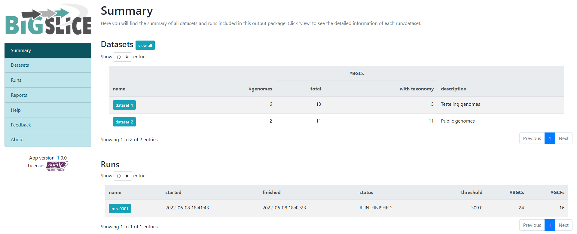
Here we have a summary of the obtained results. In the left part, we
see a set of 7 fields. 3 of them have the information that we generated:
Summary, Datasets, and Runs. The
other ones are for information regarding the software, one of them is to
give feedback to the developers. You can acces to the
Datasets and Runs page also from the options
that we see in the main part of this summary page. The first part of
this summary describes the datasets that we provided as input. The
second one is the information of the process (when we ran the program)
that BiG-SLiCE carry out with our data.
If we click into the Runs field on the left or the
run-0001 blue button on the Runs main
section, we will jump into the page that gives us the information
regarding the BGCs GCFs that were obtained:
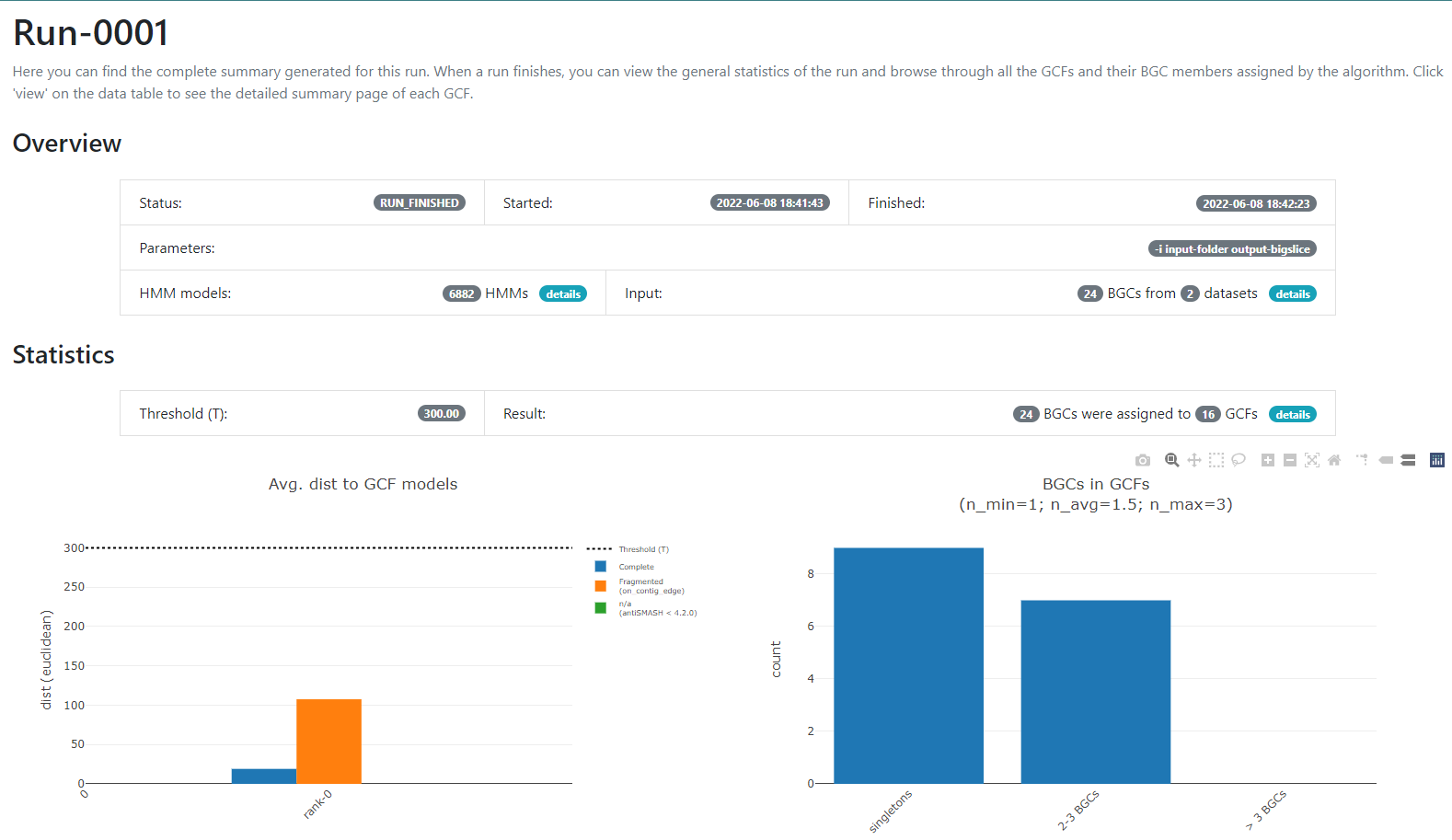
In this new page we have two bar-plots that give us information
regarding if the BGCs that we sumministrated were classified as
fragmented or complete by AntiSMASH (according to the
AntiSMASH algorithm, a BGC can be classified as fragmented
if it is found at the edge of a contig), and how many families were
obtained with singletons (composed of just one BGC) and of 2-3 BGCs.
If we go to the bottom of this page, we will found a table of all the GCFs with information of the number of BGCs that compose them, the representative BGC class inside each family, and which genus has more BGCs that belong to each family.
Click the + symbol of the GCF_7, and then on the
View button that is displayed. This will take us to a page
with statistics of the BGCs that are part of this family.
Inside this section, we can found a great amount of information
regarding the GCF_7 BGC’s. If we jump to section called
Members, we can click on the view BGC arrowers
button to get a visualization of the domains that are part of each of
the genes of these BGCs.
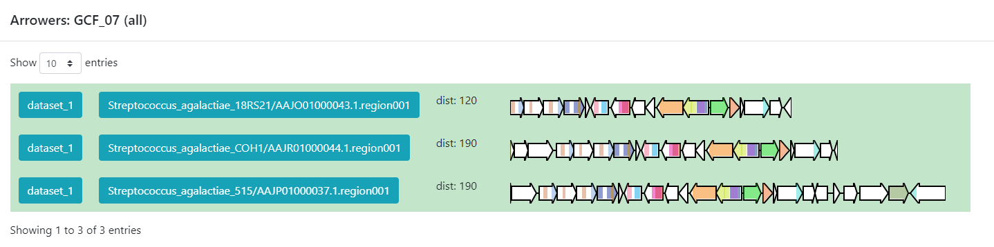
As we can see, this tool can be used to clusterize homologous BGCs that share a structure. With this knowledge, we can try some hypothesis or even build new ones in the light of this information.
Discussion
Considering the results in the runs tab, we can see that there are a
lot of Gene Cluster Families that have only one cluster associated to it
(GCF_1, GCF_2, GCF_4, GCF_5, GCF_6, GCF_8, GCF_9, GCF_13, and GCF_15).
What does this tell us about the metabolites diversity of the
Streptococcus sample?
We can see that there are some unique gene cluster families, which means that there are an organism that has that unique gene cluster and therefore it has some metabolite that the others don´t and that may be advantageous in its environment. Since there are many singleton Gene Cluster Families, we can say that there is a big diversity from the sample because many of the organisms in the sample have unique “abilities” (metabolites).
Discussion
Suppose we get the following results from a sample of 6 organisms.
|——————-+——————————————————–| | GCF | #core members | |:—————–:+:——————————————————:| | GCF_1 | 6 | |——————-+——————————————————–| | GCF_2 | 5 | |——————-+——————————————————–| | GCF_3 | 5 | |——————-+——————————————————–| | GCF_4 | 6 | |——————-+——————————————————–|
What can we infer about the metabolite diversity?
As most of the organisms have a gene cluster in the gene cluster family, we can infer that most of them have the same secondary metabolites, which means that there is little metabolite diversity between them.
BiG-FAM
To demonstrate the functionality of BiG-SLICE, the
authors gathered close to 1.2 million of BGCs. All this information,
they put it on a great database that they called BiG-FAM.
When you get to the main page, you will face a
structure that looks like the one we saw on the BiG-SLICE
results:
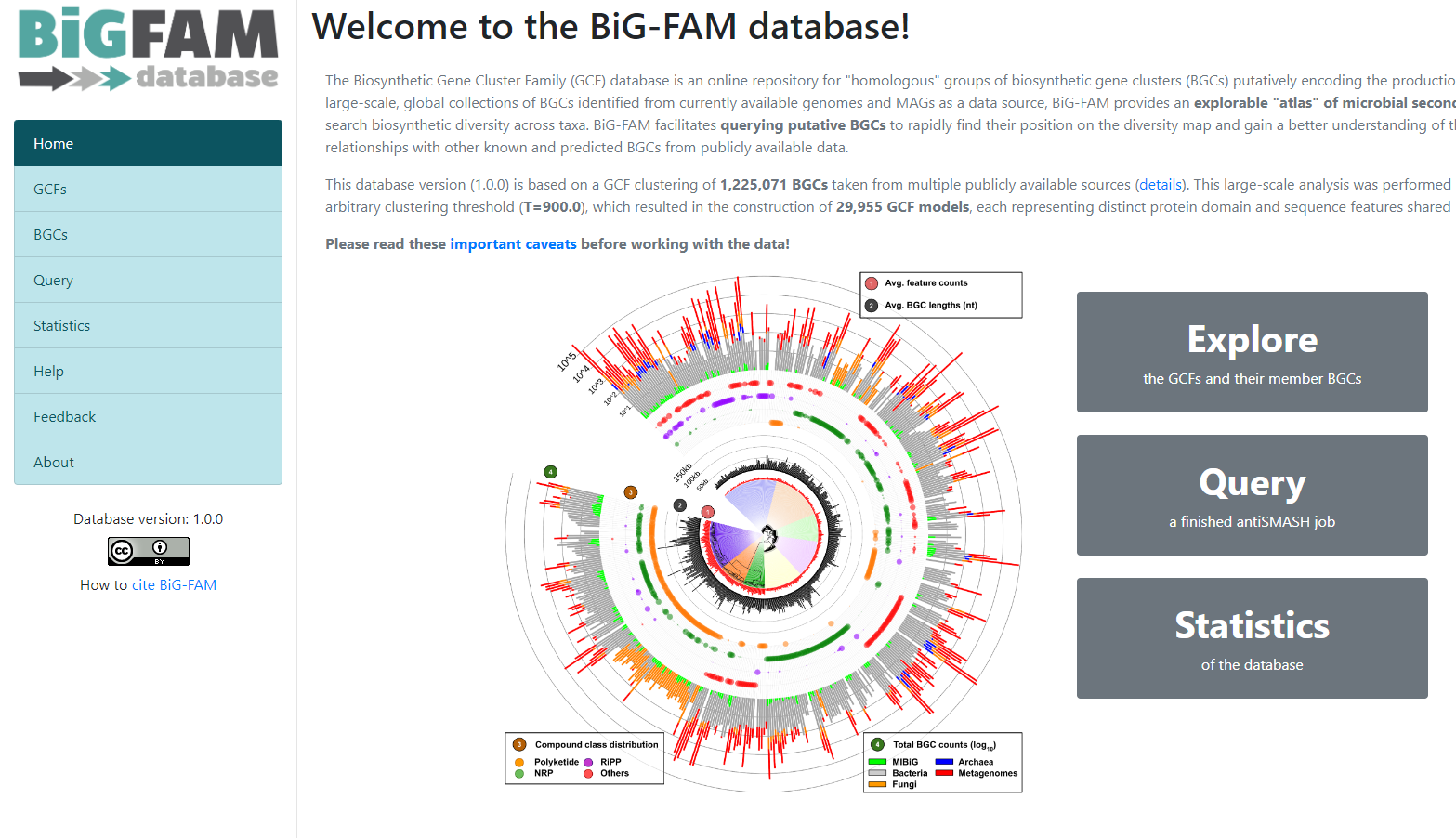
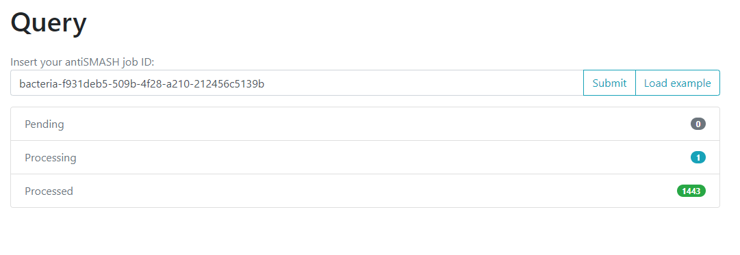
One of the options on the left is Query. If we click
here, we will move to a new page where we can insert an
antiSMASH job ID. This will run a comparison of all the
BGCs found on that antiSMASH run on a single genome, against the immense
database.
We will use the antiSMASH job ID from the analysis made
on Streptococcus agalactiae A909. The
antiSMASH job ID can be found in the URL
direction of this page in the next format:
taxon-aaaaaaa-bbbb-cccc-dddd-eeeeeeeeeeee.
We will use the job ID that we obtained:
bacteria-f931deb5-509b-4f28-a210-212456c5139b
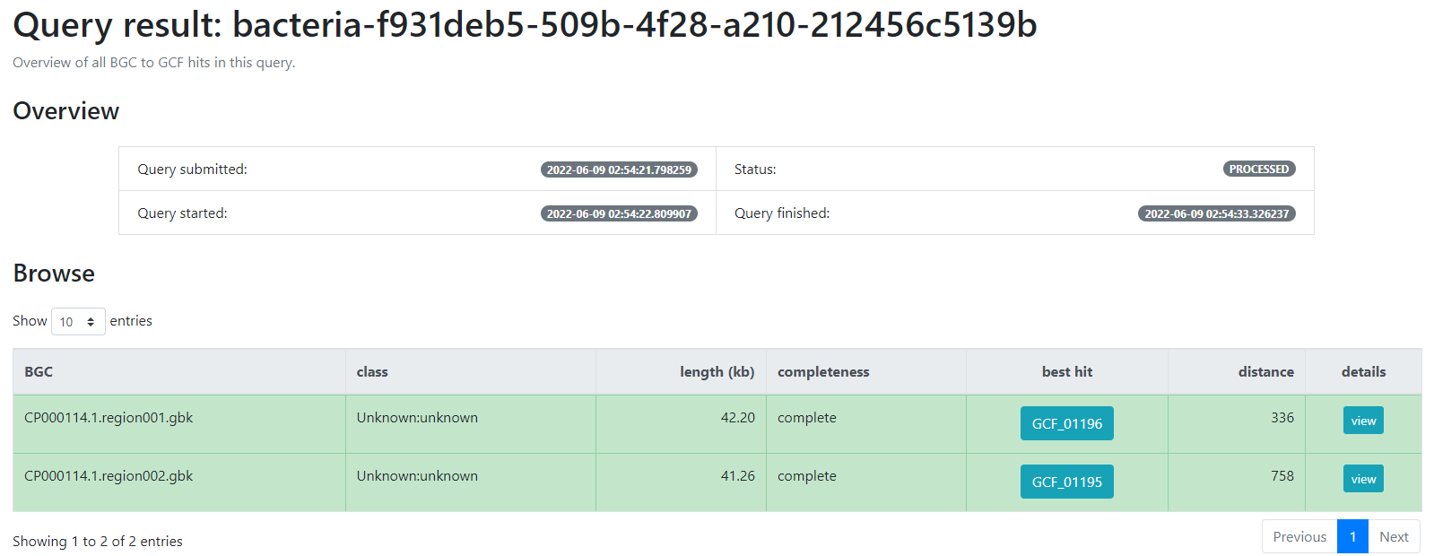
And click the submit option.
This will generate a result page that indicates with which BGCs from the database, the BGCs from the query genome are related.
-
BiG-SLiCEandBiG-FAMare softwares that are useful to compare the metabolic diversity of bacterial lineages between each other and against a big database - An input-folder containing the BGCs from antiSMASH and the taxonomic
information of each genome is needed to run
BiG-SLiCE - The results from the antiSMASH web-tool are needed to run
BiG-FAM - Gene Cluster Families can help us to compare the metabolic capabilities of a set of bacterial lineages
- We can use
BiG-FAMto compare a BGC against the whole database and predict its Gene Cluster Family
Content from Finding Variation on Genomic Vicinities
Last updated on 2026-02-20 | Edit this page
Estimated time: 35 minutes
Overview
Questions
- How can I follow variation in genomic vicinities given a reference BGC?
- Which gene families are the conserved part of a BGC family?
Objectives
- Learn to find BGC-families
- Visualize variation in a genomic vicinity
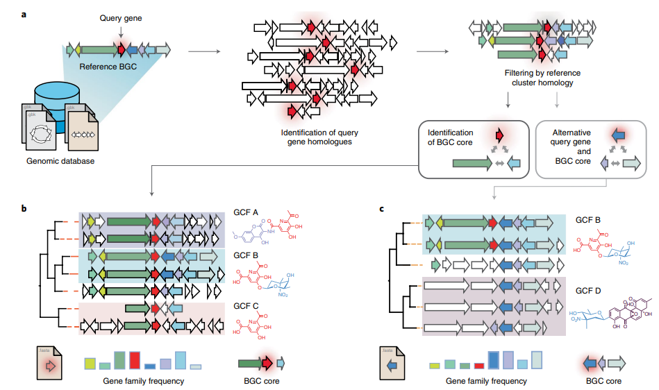
CORASON is a visual tool that identifies gene clusters that share a common genomic core and reconstructs multi-locus phylogenies of these gene clusters to explore their evolutionary relationships. CORASON was developed to find and prioritize biosynthetic gene clusters (BGC), but can be used for any kind of clusters.
Input: query gene, reference BGC and genome database. Output: SVG figure with BGC in the family sorted according to the multi-locus phylogeny of the core genes.
Advantages
- SVG graphs Scalable graphs that allow metadata easy display.
- Interactive, CORASON is not a static database, it allows to explore your own genomes.
- Reproducibility, since CORASON runs on docker and conda, the containerization allows to always perform the same analysis even if you change your Linux/perl/blast/muscle/Gblocks/quicktree local distributions.
CORASON conda
Here we are testing the new stand-alone corason in a conda environment with gbk as input-files. Firstly, activate the corason-conda environment.
OUTPUT
(corason) user@server:~$With the environment activated, all CORASON-dependencies are ready to be used. The next step is to clone CORASON-software from its GitHub repository. Firstly, place yourself at the results directory and then clone CORASON-code.
BASH
$ mkdir -p ~/pan_workshop/results/genome-mining
$ cd ~/pan_workshop/results/genome-mining
$ git clone https://github.com/miguel-mx/corason-conda.git
$ ls
The GitHub CORASON repository must be now in your directory.
OUTPUT
corason-conda Change directory by descending to EXAMPLE2. The file
cpsg.query, contains the reference protein cpsG, whose
encoding gene is part of the polysaccharide
BGC produced by some S. agalactiae
OUTPUT
cpsg.query As genomic database we will use the prokka-annotated gbk
files of S. agalactiae. This database will be stored in the
reserved directory CORASON_GENOMES.
BASH
$ mkdir  CORASON_GENOMES
$ cp ~/pan_workshop/results/annotated/Streptococcus_agalactiae_*/*gbk CORASON_GENOMES/
CORASON was written to be used with RAST annotation as input files,
in this case we are using a genome database composed of
.gbk files. Thus, we need to convert gbk files into
CORASON-compatible input files.
OUTPUT
Directory CORASON_GENOMES
../CORASON/gbk_to_fasta.pl CORASON_GENOMES agalactiae_18RS21_prokka.gbk 100001 ../CORASON
../CORASON/gbk_to_fasta.pl CORASON_GENOMES agalactiae_515_prokka.gbk 100002 ../CORASON
../CORASON/gbk_to_fasta.pl CORASON_GENOMES agalactiae_A909_prokka.gbk 100003 ../CORASON
../CORASON/gbk_to_fasta.pl CORASON_GENOMES agalactiae_CJB111_prokka.gbk 100004 ../CORASON
../CORASON/gbk_to_fasta.pl CORASON_GENOMES agalactiae_COH1_prokka.gbk 100005 ../CORASON
../CORASON/gbk_to_fasta.pl CORASON_GENOMES agalactiae_H36B_prokka.gbk 100006 ../CORASON
../CORASON/gbk_to_fasta.pl CORASON_GENOMES thermophilus_LMD-9_prokka.gbk 100007 ../CORASON
../CORASON/gbk_to_fasta.pl CORASON_GENOMES thermophilus_LMG_18311_prokka.gbk 100008 ../CORASON
Now, all converted genome files, aminoacid fasta files (.faa) and annotation files (.txt) should be placed in the ‘GENOMES directory’ one level up outside output.
OUTPUT
CORASON_GENOMES Corason_Rast.IDs cpsg.query GENOMES output Finally, we have the query enzyme, the IDs file and a genomic database of S. agalactiae in the same directory. Run CORASON with cpsg.query as query with 1000006 as an example of reference BGC.
OUTPUT
>> 100001_666.input  Cluster1237  Cluster1245  Cluster1253       cpsg.query_BGC.tre            cpsg.query_tree.svg
>> 100002_2002.input Cluster1238  Cluster1246  Cluster1254       cpsg.query.BLAST              Frequency
>> 100003_1173.input Cluster1239  Cluster1247  Cluster1255       cpsg.query.BLAST.pre          GBK
>> 100004_35.input   Cluster1240  Cluster1248  Cluster1256       cpsg.query.parser             Joined.svg
>> 100005_912.input  Cluster1241  Cluster1249  Cluster1257       cpsg.query.parser.pre         MINI
>> 100006_1247.input Cluster1242  Cluster1250  Concatenados.faa  cpsg.query_PrincipalHits.tre  PrincipalHits.muscle
>> 100007_1022.input Cluster1243  Cluster1251  CORASON           cpsg.query_Report             PrincipalHits.muscle-gb
>> 100008_1024.input Cluster1244  Cluster1252  cpsg.query        cpsg.query.svg                TempConcatenados.faa
Finally, we have all the genomic vicinities sorted phylogenetically according to the genes in the core-cluster. We can either see the output directly on the server or download the resulting svg file to our local computer. The format svg stands for scalable vector graphics, we are save it as an html file in order to get the option of open it as html. To see it in the server we must first copy the Joined.svg into Joined.html, then, go to the EXAMPLE2 directory in the r-studio files panel located at the bottom right. Once there clik in the Joined.html file and chose the option View in Web Browser. The corason figure will output in a new tab.
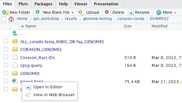
You can also use scp in a local terminal to download the
resulting svg file to your local computer.

CORASON has several installation and a conda beta versions
CORASON has one docker installation where you have to go inside the docker container, its input are RAST files. The script run_corason belongs to another installation that accepts gbk as input files. And finally, this is a beta version of CORASON conda container.
- CORASON is a command-line tool that finds BGC-families
- Genomic vicinity variation is organized phylogenetically according to the conserved genes in the BGC-family
Content from Evolutionary Genome Mining
Last updated on 2026-02-20 | Edit this page
Estimated time: 40 minutes
Overview
Questions
- What is Evolutionary Genome Mining?
- Which kind of BGCs can EvoMining find?
- What do I need in order to run an evolutionary genome mining analysis?
Objectives
- Understand EvoMining pipeline.
- Run an example of evolutionary analysis in cpsG gene family.
- Explore MicroReact interactive output interface.
Usually, bioinformatics tools related to the prediction of Natural Products (NP) biosynthetic genes try to find metabolic pathways of enzymes that are known to be related with the synthesis of secondary metabolites. However, these approaches fail for the discovery of novel biosynthetic systems. Thus, EvoMining tries to circumvent this problem by detecting novel enzymes that may be implicated in the synthesis of new natural products in Bacteria.
To know more about EvoMining you can read Selem et al, Microbial Genomics 2019.
EvoMining searches protein expansions that may have evolved from the conserved metabolism into a specialized metabolism. It builds phylogenetic trees based on all the protein copies of a certain enzyme in a given genome database. The output tree differentiates copies that are related with the conserved metabolism, copies that are known to be implicated in discovered NP-producing-BGCs i.e. BGCs from MiBIG database and, optionally, protein copies that belong to BGCs predicted by antiSMASH. Finally, some branch in the tree will be depicted as “EvoMining hits”, which represent enzyme expansions that are evolutionary closer to those copies related with the secondary metabolism (MiBIG or antiSMASH BGCs) than to those related with the conserved (primary) metabolism.
Run evomining image
First, place yourself at your working directory.
OUTPUT
CORASON_GENOMES Corason_Rast.IDs cpsg.query GENOMES outputThe general structure of a docker container is shown in the next
bash-box. Note that it requires to specify which docker container will
run. Optionally, with -v flag it is possible to share a
directory with the container, with -p flag a port is shared
and it is also possible to specify which program will run inside the
container.
BASH
$ docker run --rm -i -t -v <your local directory>:<inside docker directory> -p <inside port>:80 <docker container> <program inside docker> EvoMining is inside a docker container, so the general structure to start your analysis will be as follows:
BASH
$ docker run --rm -i -t -v $(pwd):/var/www/html/EvoMining/exchange -p 8080:80 nselem/evomining:latest /bin/bash Let’s explain the pieces of this line.
| command | Explanation |
|---|---|
| docker | tells the system that we are running a docker command |
| run | the command that we are running is to run a docker container |
| --rm | this container will be removed after closed |
| -i | this container allows user interaction |
| -t | this interaction will be through a terminal |
| -v | a data volume (directory) will be shared between your local machine and the container |
| -p | a port will allow a web based app |
However, sometimes the port 80 is busy, in that case you can use
other ports like 8080 or 8084. If this is the case, please use the port
80X where X is a number between 01..30 provided by your
instructor.
BASH
$ docker run --rm -i -t -v $(pwd):/var/www/html/EvoMining/exchange -p 8080:80 nselem/evomining:latest /bin/bash
$ docker run --rm -i -t -v $(pwd):/var/www/html/EvoMining/exchange -p 8084:80 nselem/evomining:latest /bin/bash
If your docker container worked, now you will see in your terminal a
new prompt. Instead of the usual dollar sign, there should be a number
# at the beginning of your terminal. This is because now
you are inside the docker container and you have sudo
permissions inside the docker.
To exit container use exit
And now your prompt must be back in the dollar sign
Set EvoMining genomic database
Start the container again with your corresponding port.
BASH
$ docker run --rm -i -t -v $(pwd):/var/www/html/EvoMining/exchange -p 80X:80 nselem/evomining:latest /bin/bash Though we will NOT run the test EvoMining command, it looks as follows:
# perl startEvoMining.pl Instead of that, customize the genomic database by using the same as
CORASON.
Notice that EvoMining requires RAST-like annotated genomes and for this
reason we are using the fasta files that CORASON converts from our gbk
inputs.
# perl startEvoMining.pl -g GENOMES -r Corason_Rast.IDs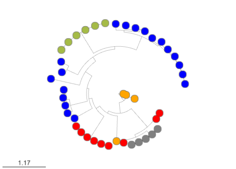

Finally, remember that X means your user-number and open
your browser at the address:
http://132.248.196.38:80X/EvoMining/html/index.html. Once
there, just click the start button and enjoy! (click on the submit
buttons!)
When you finish using this container, please exit it.
#exitVisualize your results in MicroReact
Firstly, you have to run all the pipeline in the website: http://
EvoMining outputs are stored in the directory
<conserved-db>_<natural-db>_<genomes-db>
To explore EvoMining outputs, you need to upload 1.nwk and 1.csv files to microReact. There are many methods to download files from the server to your local computer.
If you are using JupyterHub you explore the file folders and select the files and then press the download button.
You can use the export button in the file panel of R studio. To
download the files, first in the files panel open in the directory
~/pan_workshop/results/genome-mining/corason-conda/EXAMPLE2/ALL_curado.fasta_MiBIG_DB.faa_GENOMES/blast/seqf/tree,

Then, select files 1.nwk and 1.csv in that directory, click
more in the engine icon, and select the export
option in the menu. The files will be downloaded to your local computer,
and now you will be able to upload them to MicroReact.
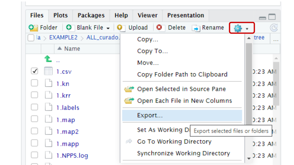
Alternatively, If your prefer to use the terminal to download files
the scp protocol can download the files into your local
machine.
BASH
scp betterlab@132.248.196.38:~/pan_workshop/results/genome-mining/corason-conda/EXAMPLE2/ALL_curado.fasta_MiBIG_DB.faa_GENOMES/blast/seqf/tree/1.nwk ~/Downloads/.
scp betterlab@132.248.196.38:~/pan_workshop/results/genome-mining/corason-conda/EXAMPLE2/ALL_curado.fasta_MiBIG_DB.faa_GENOMES/blast/seqf/tree/1.csv ~/Downloads
Here you can find the MicroReact visualization of this EvoMining run.
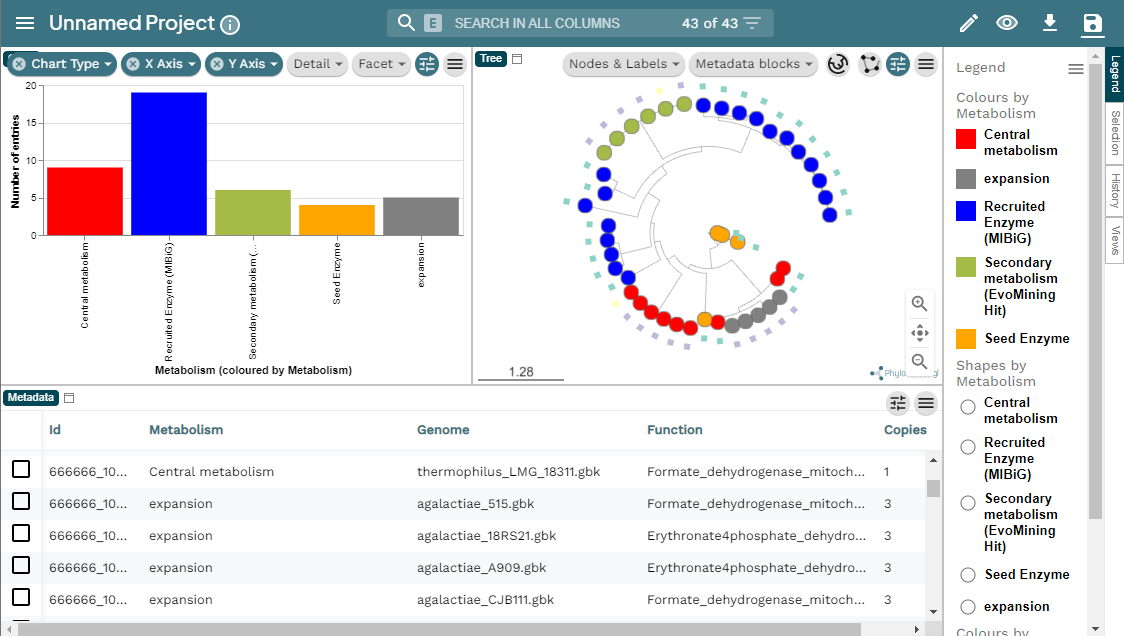
Other resources
To run EvoMining with a larger conserved-metabolite DB you can use EvoMining Zenodo data.
To explore more EvoMining options, please explore EvoMining wiki.
Set the conserved-enzymes database
When using EvoMining, oftenly you will desire to construct your own conserved enzymes database. To know more about how to configure a database, consult the EvoMining wiki in the EvoMining databases part. Natural products database could also be replaced for another set of genes that are “true positives”, for example a set of regulatory genes.
As an example, transform the file cpsg.query into the
format of this database. This file contains the aminoacid sequence of
the cpsG gene. Firstly, copy this file into what will become
the conserved-enzymes database.
Now, it requires some editing. Open nano editor and change the first
line >cpsg to
>SYSTEM1|1|phosphomannomutase|Saga. EvoMining
conserved-database needs a four-field format pipe-separated that
contains; the name of the metabolic system to which the enzyme belongs
(SYSTEM1), a consecutive number of the enzyme (1 in this case), the
function of the enzyme, and finally, an abbreviation of the organism
Saga, (S. Agalactiae).
The reason behind this is that this was the way we needed EvoMining for
its first use and we have not changed the headers since.
OUTPUT
>SYSTEM1|1|phosphomannomutase|Saga
MIFVTVGTHEQQFNRLIKEVDRLKGTGAIDQEVFIQTGYSDFEPQNCQWSKFLSYDDMNSYMKEAEIVITHGGPATFMSVISLGKLPVVVPRRKQFGEHINDHQIQFLKKIAHLYPLAWIED
Run your EvoMining docker
BASH
$ docker run --rm -i -t -v $(pwd):/var/www/html/EvoMining/exchange -p 80X:80 nselem/evomining:latest /bin/bash and inside this new container:
# perl startEvoMining.pl -g GENOMES -r Corason_Rast.IDs -c cpsg_cdbUse the website again and think about the results.
Exercise 1. Set EvoMining parameters
Complete the blanks in the following EvoMining run:
actinoSMASH A file with the ids of antiSMASH recognized
genes. Actinos a directory with RAST-like fasta and
annotation files. Histidine-db A fasta file with some
proteins in the histidine pathway.Actinos.ids tabular files with the RAST ids and the name of
the organisms.
# perl starEvoMining.pl -g ____ -c _____ -r _____ -a ___________ Discussion 1. Retro EvoMining in enzyme database
What do you learn from running in a conserved-enzymes database the gene cpsG that is part of a specialized BGC?
cpsG does not have extra copies in Streptococcus agalactiae, so there are no expansions that may be functional divergent. cpsG single copies in the genomes look red-colored in EvoMining output, as if they belong to the conserved-metabolism. However, this is not the case, the color is because there is only one copy and it is merged into MIBiG true-positives because it was originally a gene in the specialized metabolism. So it is important to know the seed enzymes.
OUTPUT
cpsg_cdb_MiBIG_DB.faa_GENOMESARTS is another evolutionary genome mining software with its corresponding database ARTS-db .
Evolutionary Genome Mining
To learn more about Genome Mining you can read these references:
- The confluence of big data and evolutionary genome mining for the discovery of natural products. Chevrette et al, 2021`
- Evolutionary Genome Mining for the Discovery and Engineering of Natural Product Biosynthesis. Chevrette et al, 2022
More about docker
To see the running container use
ps
If there are containers in use you will see a list of all of them.
OUTPUT
2f879ba6e337 nselem/evomining:latest "/bin/bash" 11 hours ago Up 11 hours 0.0.0.0:8014->80/tcp, :::8014->80/tcp relaxed_dirac
- EvoMining is a command-line tool that performs evolutionary genome mining over gene families
- EvoMining hits can belong to new BGC
- MicroReact is an interactive genomic visualizer compatible with EvoMining output
Content from GATOR-GC: Genomic Assessment Tool for Orthologous Regions and Gene Clusters
Last updated on 2026-02-20 | Edit this page
Estimated time: 60 minutes
Overview
Questions
- What is GATOR-GC, and how does it differ from other BGC exploration tools?
- How does GATOR-GC establish BGC boundaries using evolutionary principles?
- What types of biosynthetic diversity can GATOR-GC identify?
- What do I need to perform a targeted exploration using GATOR-GC?
Objectives
- Understand the GATOR-GC algorithm and its evolutionary approach to BGC boundary definition.
- Learn how to conduct a targeted search for key enzymes within BGCs and genomic islands using GATOR-GC.
- Execute an example analysis using customizable parameters for precision in identifying GATOR windows.
- Visualize and interpret the output of GATOR-GC, including gene cluster diagrams and genomic neighborhoods.
![]()
GATOR-GC is a user-friendly algorithm designed for targeted exploration of BGC and genomic islands diversity. It focuses on key biosynthetic enzymes and offers flexibility in defining the taxonomic scope of the analysis. Unlike methods relying on arbitrary cutoffs, GATOR-GC establishes BGC boundaries based on evolutionary principles and implements an enzyme-aware scoring system for assessing BGC-BGC distances, moving beyond a binary presence-absence framework. This approach enhances the tool’s capability to identify and prioritize novelty, effectively mapping biosynthetic diversity into distinct groups.
To know more about GATOR GC you can go to the Github repository.
Most relevant features
- Targeted Search: Conduct targeted searches for essential key enzymes and optional tailor enzymes within Biosynthetic Gene Clusters (BGCs) and genomic islands, streamlining the discovery process.
- Modular Domain Screening: Automatically screen user-provided protein files to identify critical modular domains, such as Non-Ribosomal Peptide Synthetases (NRPSs) and Polyketide Synthases (PKSs), using state-of-the-art HMM profiles from antiSMASH for unparalleled precision.
- Customizable Parameters: Customize search parameters to include required and optional proteins, ensure complete assembly with all necessary proteins, and define specific distances between required proteins. This customization enhances the specificity of GATOR window identification, offering tailored analysis to meet research needs.
- Dereplication for Gator Windows: Remove identical Gator Windows to avoid redundant calculations in subsequent steps, while keeping track of which windows are duplicates
- GATOR Focal Scores: Employ a novel enzyme-aware scoring system to accurately compare GATOR windows against targeted focal windows. This approach ensures precise evaluation of genomic contexts and enzyme functionalities.
- GATOR Conservation: Generate dynamic gene cluster diagrams that visually differentiate between required and optional proteins using color coding. Transparency levels indicate the gene’s presence within GATOR windows, providing a clear visual representation of gene conservation
- GATOR Neighborhoods: Visualize each GATOR window’s genomic neighborhood with organized tracks based on GATOR focal scores. Homology between genes is intuitively illustrated with gray bars, facilitating easy understanding of genetic relationships and conservation

GATOR GC
Before starting, make sure to activate the gator-gc
environment.
The first part of running GatorGC has to do with creating a database. To facilitate the process first we need to create a directory where we can find all Gator-GC results:
After creating this, we will move to this folder
To create the database, we need all the annotated genomes that we
have previously processed. For the database, we only require the genbank
files, which end with gbk. We can use the cp command to
copy all the genbank files of our annotated genomes to a folder in this
directory. First, we will create the directory where we will copy the
files.
Exercise 1. Copy all the gbk files to the new directory
We know that all the genbank files are in the following path
~/pan_workshop/results/annotated/ and inside the annotated
folder, there is a folder for each genome and each folder contains the
output files from prokka. You can use
tree ~/pan_workshop/results/annotated/to confirm this.
Using cp, try to complete the gaps in the following command
to copy all the genbank files from the previously processed genomes to
the new directory you created gbks. Remember you can use
* to match any symbol(s).
Set GATOR-GC database
Now that we have the genbank files in a folder we can create the
necessary database for gator-gc. The command to create the database is
pre-gator-gc. You can use the -h flag to
explore the options of this command.
OUTPUT
usage: pre-gator-gc [-h] -g  [...] [-e] [-t] -o  [-v]


     -\ ---\--\ -------\ ----\ ---\--\ ---\ --\ ----\ ----\--------\ /---
   /--/ ---/--/ -------/ ----/ ---/--/ ---/ --/ ----/ ----/--------/ \----\
  ________   _____  __________________  __________         _________________
 /  _____/  /  _  \ \__    ___/_____  \ \______   \       /  _____/\_   ___ \
/   \  ___ /  /_\  \  |    |   /   |   \ |       _/ _____    \  ___/    \  \/
\    \_\  \    |    \ |    |  /    |    \|    |   \/_____/    \_\  \     \_____
 \______  /____|__  / |____|  \_______  /|____|_  /       \______  /\_______  /
        \/        \/                  \/        \/               \/         \/
    -----\--\ -------\ ----\ ---\--\ ---\ --\ ------\ ----\---------\ /----
    \----/--/ -------/ ----/ ---/--/ ---/ --/ ------/ ----/---------/ \----/

GATOR-GC: Genomic Assessment Tool for Orthologous Regions and Gene Clusters
Developer: José D. D. Cediel-Becerra
Afiliation: Microbiology & Cell Science Deparment, University of Florida
Please contact José at jcedielbecerra@ufl.edu if you have any issues
Version: v0.9.0

optional arguments:
  -h, --help  show this help message and exit
  -v          Enable verbose output (default: False).

Input Options:
  -g  [ ...]  Directories containing GenBank files (*.gbff/*.gbk/*.gb). You can specify multiple directories separated by spaces. Directories can be specified with or without wildcards.

HMMER Options:
  -e          E-value threshold for HMMER hmmsearch (default: 1e-4).
  -t          Number of CPU threads to use for hmmsearch (default: all available threads).

Output Options:
  -o          Directory where the gator databases (protein,  DIAMOND, and modular domtblout databases) will be saved.
As we can see in the help output, we have to feed the command with -g which is the path to the folder containing the genbank files and -o which is the directory where we want gator to save the database to be processed (output folder). To create the database we will use the following line of code:
OUTPUT
     -\ ---\--\ -------\ ----\ ---\--\ ---\ --\ ----\ ----\--------\ /---
   /--/ ---/--/ -------/ ----/ ---/--/ ---/ --/ ----/ ----/--------/ \----\
  ________   _____  __________________  __________         _________________
 /  _____/  /  _  \ \__    ___/_____  \ \______   \       /  _____/\_   ___ \
/   \  ___ /  /_\  \  |    |   /   |   \ |       _/ _____    \  ___/    \  \/
\    \_\  \    |    \ |    |  /    |    \|    |   \/_____/    \_\  \     \_____
 \______  /____|__  / |____|  \_______  /|____|_  /       \______  /\_______  /
        \/        \/                  \/        \/               \/         \/
    -----\--\ -------\ ----\ ---\--\ ---\ --\ ------\ ----\---------\ /----
    \----/--/ -------/ ----/ ---/--/ ---/ --/ ------/ ----/---------/ \----/

GATOR-GC: Genomic Assessment Tool for Orthologous Regions and Gene Clusters
Developer: José D. D. Cediel-Becerra
Afiliation: Microbiology & Cell Science Deparment, University of Florida
Please contact José at jcedielbecerra@ufl.edu if you have any issues
Version: v0.9.0
[1] - 2024-08-20 14:06:32,797 - INFO - The gator_databases directory was created successfully.
[2] - 2024-08-20 14:06:32,797 - INFO - Total genome files found: 9
[3] - 2024-08-20 14:06:34,223 - INFO - Successfully created the gator protein database to gator_databases/gator_databases.faa
[4] - 2024-08-20 14:06:34,295 - INFO - Successfully created the gator DIAMOND database to gator_databases/gator_databases.dmnd
[5] - 2024-08-20 14:06:34,946 - INFO - Successfully created the gator domtblout database to gator_databases/gator_databases.domtblout
[6] - 2024-08-20 14:06:34,946 - INFO - Execution time: 2.15 secondsQUESTION: You already read the help page of
pre-gator-gc. Why we added the flag -v?
GATOR-GC
Now that we have the database ready, let’s review what we need to run
gator-gc. To find out, we can type the command with the
-h help flag.
OUTPUT
usage: gator-gc [-h] -rq  [-op] -g  [...] -d  [-t] [-qc] [-idt] [-e] [-rd] [-we] -o  [-nc] [-nn] [-v]

     -\ ---\--\ -------\ ----\ ---\--\ ---\ --\ ----\ ----\--------\ /---
   /--/ ---/--/ -------/ ----/ ---/--/ ---/ --/ ----/ ----/--------/ \----\
  ________   _____  __________________  __________         _________________
 /  _____/  /  _  \ \__    ___/_____  \ \______   \       /  _____/\_   ___ \
/   \  ___ /  /_\  \  |    |   /   |   \ |       _/ _____    \  ___/    \  \/
\    \_\  \    |    \ |    |  /    |    \|    |   \/_____/    \_\  \     \_____
 \______  /____|__  / |____|  \_______  /|____|_  /       \______  /\_______  /
        \/        \/                  \/        \/               \/         \/
    -----\--\ -------\ ----\ ---\--\ ---\ --\ ------\ ----\---------\ /----
    \----/--/ -------/ ----/ ---/--/ ---/ --/ ------/ ----/---------/ \----/

GATOR-GC: Genomic Assessment Tool for Orthologous Regions and Gene Clusters
Developer: José D. D. Cediel-Becerra
Afiliation: Microbiology & Cell Science Deparment, University of Florida
Please contact José at jcedielbecerra@ufl.edu if you have any issues
Version:v0.9.0

optional arguments:
  -h, --help  show this help message and exit
  -v          Enable verbose output. (Default: False)

Input Options:
  -rq         Path to the query protein FASTA file containing required proteins.
  -op         Path to the query protein FASTA file containing optional proteins.
  -g  [ ...]  Directory containing the Genbank files (*.gbff/*.gbk/*.gb).You can specify multiple directories separated by spaces. Directories can be specified with or without wildcards.
  -d          Directory containing the PRE-GATOR-GC databases (.dmnd and .domtblout files). (Required)

Diamond Options:
  -t          Number of CPUs to use for diamond search and hmmsearch. (Default: all available CPUs)
  -qc         Minimum percent query cover for diamond search. (Default: 70)
  -idt        Minimum percent identity for diamond search. (Default: 35)

HMMER Options:
  -e          E-value threshold for hmmsearch. (Default: 1e-4)

GATOR-GC Options:
  -rd         Maximum distance in kilobases between required genes to define a gator window. (Default: 86 kb)
  -we         Extension in kilobases from the start and end positions of the gator windows. (Default: 10 kb)

Output Options:
  -o          Directory to save GATOR-GC results.
  -nc         Disable creation of GATOR conservation figures.
  -nn         Disable creation of GATOR neighborhoods figures.
From this output, we can see the Gator-GC options. The minimum requirements to run gator-gc are:
-
-rqPath to the query protein FASTA file containing required proteins. -
-gDirectory containing the Genbank files. -
-dDirectory containing the PRE-GATOR-GC databases. -
-oOutput directory
To compare the results obtained by the different tools we have used,
we will use the reference protein cpsG, whose encoding gene is part of
the polysaccharide BGC produced by some S. agalactiae. The
aminoacid fasta is already in the server in
~/pan_workshop/results/genome-mining/corason-conda/EXAMPLE2/cpsg.query.
So the command to run gator-gc is the following:
BASH
$ gator-gc -rq ~/pan_workshop/results/genome-mining/corason-conda/EXAMPLE2/cpsg.query -g gbks/ -d gator_databases/ -o cpsg_gatorOnce Gator-GC finishes, we can observe the structure of the files
created by the program using tree.
OUTPUT
cpsg_gator/
├── all_merged_queries_38nh2fip.faa
├── all_merged_queries_unvwb3pq.domtbl
├── allvall_proteins_nuxdlir7.faa
├── concatenated_scores
│   ├── clustermap_gfs.svg
│   └── concatenated_gfs.csv
├── deduplicate_allvall_proteins_e3svhd1_.faa
├── deduplicate_dmnd_db__lno1x3_.dmnd
├── deduplicate_dmnd_out_3ve4lo6v.dmnd
├── deduplication_data
│   ├── deduplication_gfs.csv
│   └── unq_comp.tsv
├── dmnd_db_r0qpquhc.dmnd
├── dmnd_out_aun2m_k5.txt
├── gator_conservation_plots
│   ├── window_1--Streptococcus_agalactiae_2603V_prokka.svg
│   ├── window_2--agalactiae_515_prokka.svg
│   ├── window_4--Streptococcus_agalactiae_COH1_prokka.svg
│   ├── window_5--Streptococcus_agalactiae_CJB111_prokka.svg
│   ├── window_8--Streptococcus_agalactiae_NEM316_prokka.svg
│   └── window_9--Streptococcus_agalactiae_18RS21_prokka.svg
├── gator_neighborhoods_plots
│   ├── window_1--Streptococcus_agalactiae_2603V_prokka_neighborhoods.svg
│   ├── window_2--agalactiae_515_prokka_neighborhoods.svg
│   ├── window_4--Streptococcus_agalactiae_COH1_prokka_neighborhoods.svg
│   ├── window_5--Streptococcus_agalactiae_CJB111_prokka_neighborhoods.svg
│   ├── window_8--Streptococcus_agalactiae_NEM316_prokka_neighborhoods.svg
│   └── window_9--Streptococcus_agalactiae_18RS21_prokka_neighborhoods.svg
├── gator_scores
│   ├── window_1--Streptococcus_agalactiae_2603V_prokka_GFS.csv
│   ├── window_2--agalactiae_515_prokka_GFS.csv
│   ├── window_4--Streptococcus_agalactiae_COH1_prokka_GFS.csv
│   ├── window_5--Streptococcus_agalactiae_CJB111_prokka_GFS.csv
│   ├── window_8--Streptococcus_agalactiae_NEM316_prokka_GFS.csv
│   └── window_9--Streptococcus_agalactiae_18RS21_prokka_GFS.csv
├── non_modular_queries_82tvei7d.faa
├── presence_absence
│   ├── window_1--Streptococcus_agalactiae_2603V_prokka.csv
│   ├── window_2--agalactiae_515_prokka.csv
│   ├── window_4--Streptococcus_agalactiae_COH1_prokka.csv
│   ├── window_5--Streptococcus_agalactiae_CJB111_prokka.csv
│   ├── window_8--Streptococcus_agalactiae_NEM316_prokka.csv
│   └── window_9--Streptococcus_agalactiae_18RS21_prokka.csv
└── windows_genbanks
    ├── gator_hits.tsv
    ├── window_1--Streptococcus_agalactiae_2603V_prokka.gbk
    ├── window_2--agalactiae_515_prokka.gbk
    ├── window_3--Streptococcus_agalactiae_A909_prokka.gbk
    ├── window_4--Streptococcus_agalactiae_COH1_prokka.gbk
    ├── window_5--Streptococcus_agalactiae_CJB111_prokka.gbk
    ├── window_6--Streptococcus_agalactiae_H36B_prokka.gbk
    ├── window_7--Streptococcus_agalactiae_515_prokka.gbk
    ├── window_8--Streptococcus_agalactiae_NEM316_prokka.gbk
    └── window_9--Streptococcus_agalactiae_18RS21_prokka.gbk

7 directories, 47 files
The output folder cpsg_gator/ for gator-gc includes the
following subfolders:
- windows_genbanks: This folder contains GenBank files, each generated for a specific window.
- presence_absence: Within this folder, you can find gene-level presence-absence tables for each gator window in CSV format. The tables are named based on the window number and the corresponding GenBank filename.
- gator_scores: This folder houses tables with a structure similar to the presence-absence tables. However, instead of binary numbers, normal distributions were applied to each protein. The highest distribution value is set to 1, and these values were multiplied by the presence-absence values.
- concatenated_scores: This folder contains a CSV file, which consolidates all the gator focal scores. Additionally, a “clustermap_GFSs” file displays the distribution of gator windows based on the gator focal scores using a heatmap and a dendrogram.
Here is the resulting heatmap and dendrogram. You can view the images in the file explorer on the left side of the server screen. Remember to go to the specific folder to open the file.

- gator_conservation_plots: This folder includes high-quality vectorized figures, each corresponding to a gator focal window. These figures display the gene organization and cluster size. The figure corresponding to the first window is shown below:

In these figures required genes are represented in purple, optional genes in orange, and genes not present in the protein queries files in green. The transparency of each gene’s color is determined by the conservation of homologous genes found in the gator windows.
- gator_neighborhoods_plots: Here you can find high-quality vectorized figures showcasing genome neighborhoods. Each file corresponds to a gator focal window (top track), with the remaining gator windows sorted based on the gator focal scores. This arrangement positions the second top track as the most similar gator window, and the last track at the bottom represents the most dissimilar gator window. The genomic organization of the gator windows is flipped based on the first required gene in the gator focal window, ensuring that the genomic organization aligns with that of the gator focal window. Homology rails are displayed, depicting the diamond protein alignment position hits in the genes. The first one shoul look like this:

- GATOR-GC is an innovative tool that uses an enzyme-aware scoring system and evolutionary principles to explore BGC diversity.
- Unlike traditional methods, GATOR-GC offers flexibility in defining the taxonomic scope and prioritizes the identification of novel biosynthetic pathways.
- GATOR-GC can be customized to search for essential and optional enzymes, making it a powerful tool for targeted exploration.
- Dynamic gene cluster diagrams and GATOR neighborhood visualizations provide clear insights into gene conservation and genomic relationships.
Content from Metabolomics workshop
Last updated on 2026-02-20 | Edit this page
Estimated time: NA minutes
Overview
Questions
- How can I evaluate the similarity between MS spectra?
Objectives
- Understand how GNPS molecular networks work.
- Use raw mzML metabolomic data for annotation.
- Visualize and explore molecular networks
Introduction
In the previous sections, we explored the biosynthetic potential of various strains by analyzing the BGCs within their genomes. We utilized BiG-SCAPE to create BGC networks, which compare all the BGCs detected by antiSMASH to determine their relatedness. Similarly, using metabolomics we can investigate the metabolites produced by selected strains in the laboratory. While crude extracts can be made to analyze the metabolites of specific strains, it is also possible to study the metabolites present in complex samples, such as soil, marine environments, host organisms, or stool samples. There are two approaches to annotating metabolomics data. The first comprises using the information obtained by LC-MS, comparing the exact mass and UV spectra of each detected metabolite through natural product databases. The introduction of the global natural products social molecular networking GNPS platform for molecular networking (M. Wang et al., 2016), significantly influenced dereplication techniques. Molecular networking groups metabolites into molecular families (MFs), thereby improving the annotation process of unknown metabolites.
](../fig/Molecular-network.png)
Creating a GNPS account
Before starting this tutorial, it will be useful to have a GNPS account. For that go to the GNPS webpage and select Create a new account.
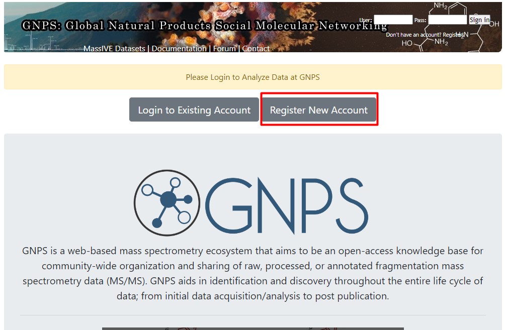
Then fill in the following information:
- Username
- Name
- Organization
- Password
Wait for a confirmation email, and you now have a GNPS account.
Download MZMine v3.9
First, go to the MZMine 3.9 release MZMine 3.9
Select the installable file depending on your computer
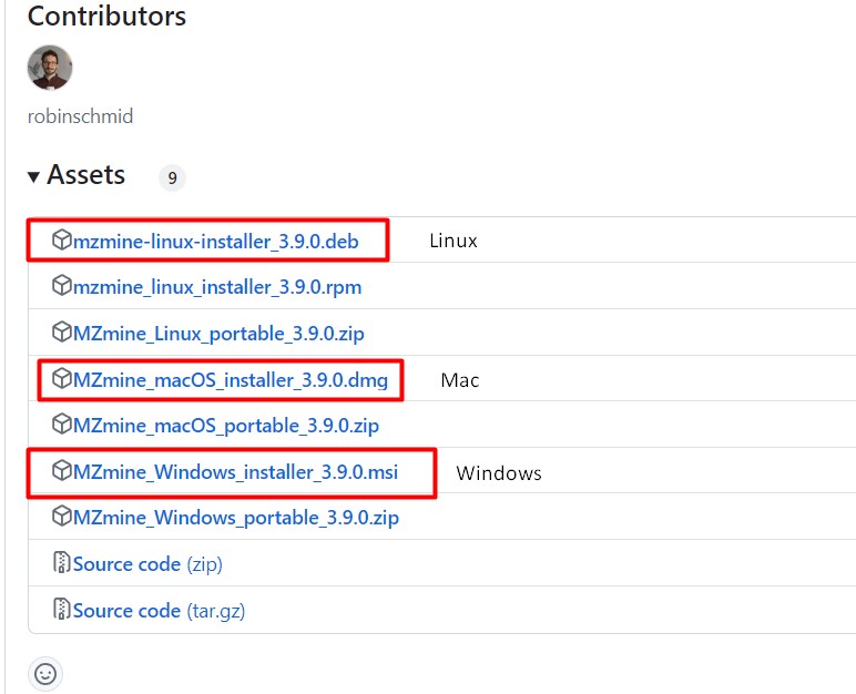
- Double-click on the file, and install the software
Download Cytoscape
Cytoscape is a software frequently used to visualize networks, such as BGC networks or molecular networks.
Go to Cytoscape webpage
Click on download Cytoscape for your operating system
Install Cytoscape in your computer.
Download the metabolomics dataset
First, we need to go to Zenodo and download all the mzML raw data collected from the described strains. https://zenodo.org/api/records/13352458/files-archive
After downloading the compressed file, we need to decompress it and store the files in a folder on our computer.
Import the dataset, and use the batch file to analyze your data
This data was collected from crude extracts from two marine Streptomyces: Streptomyces sp. H-KF8, and Streptomyces sp. Vc74B-19. Two media were used, ISP2 and ISP2 prepared with artificial seawater (ASW), to evaluate the effect of replicating the natural environment from which these strains were isolated.
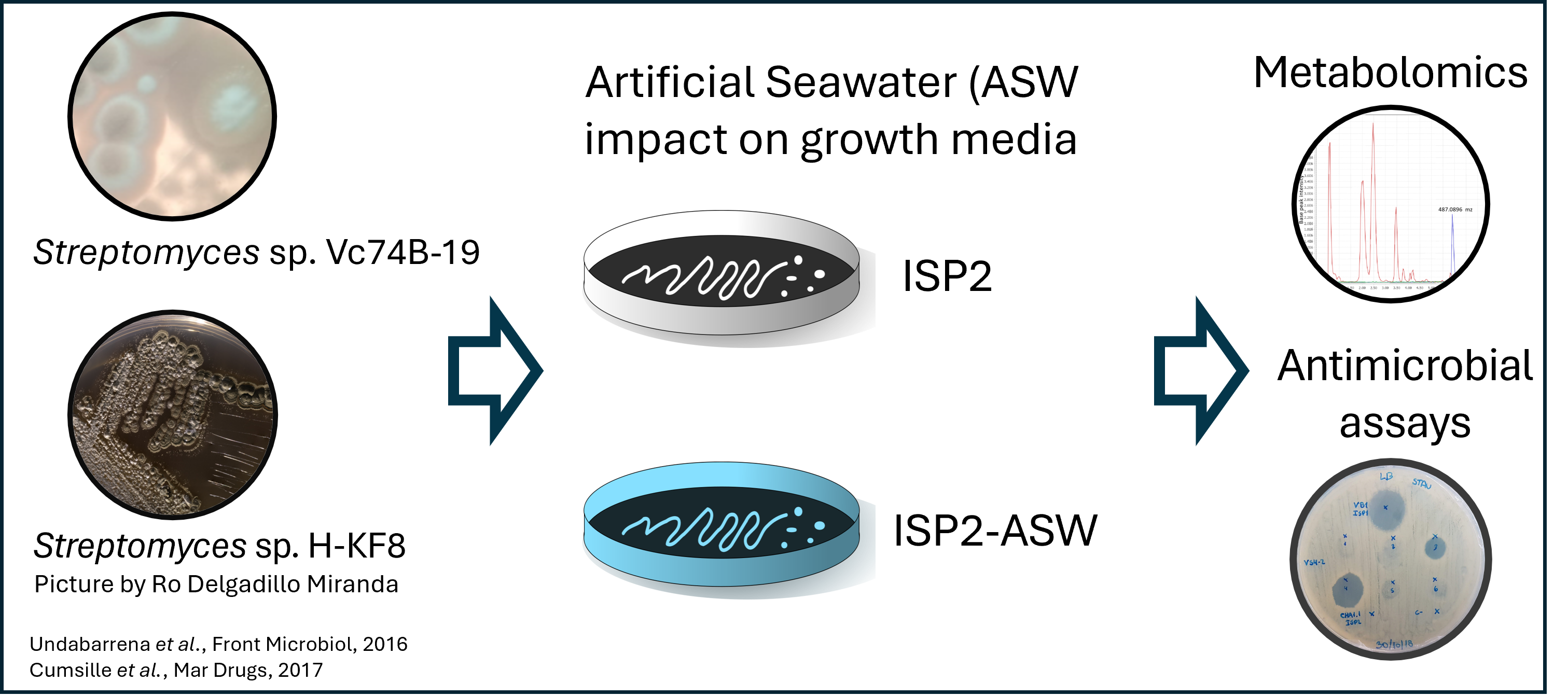
We downloaded 18 LC-MS/MS-derived files in mzML format. This data was collected by Dr. Mauricio Caraballo-Rodriguez in the Dorrestein Lab, at the University of California San Diego. There are files from each strain, in ISP2 and ISP2-ASW, besides the crude extracts from the culture media. The data is in triplicates.
Besides mzML files, there is a file metadata_table.tsv, that contains all the relevant information from this dataset. Includes the names of the samples, relevant data collection, and taxonomic information.
In addition, there is information relevant to the analysis, such as the names of the strains, the media used for culturing, and the antimicrobial activity. All this information is included in the format ATTRIBUTE_*
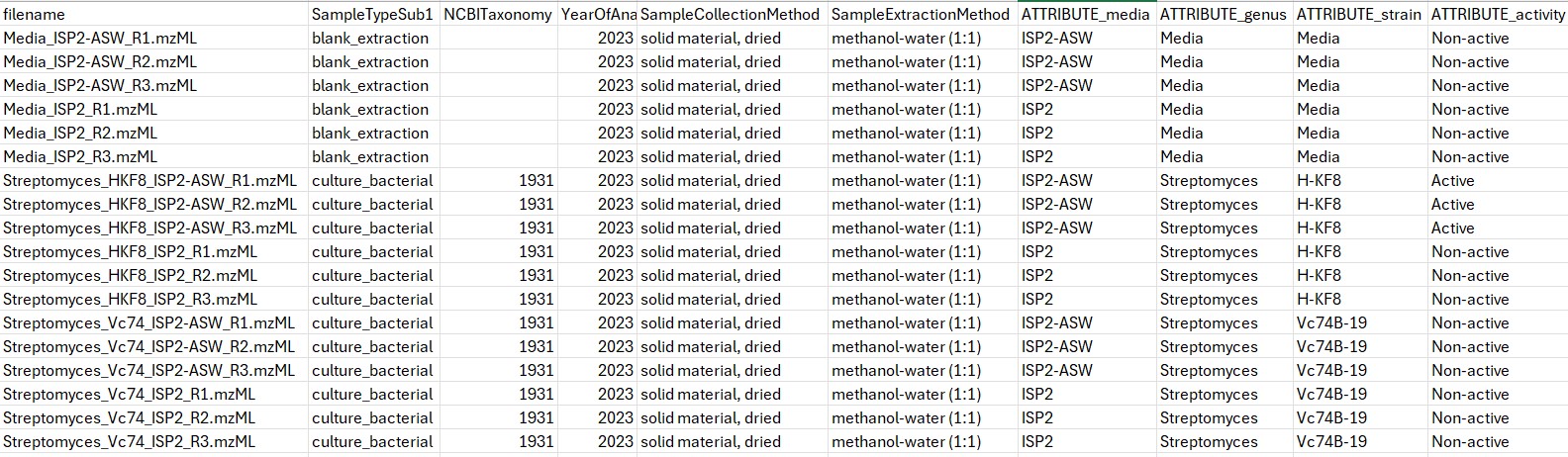
At last, there is a file named MZMine_FBMN_batch.xml that collects all the information necessary for the analysis using MZMine
Analysis using MZMine
Load batch file
Open MZMine3, click on “Open”, and then in “Batch Mode”
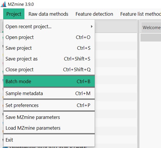
Here you should select load, and search for your downloaded files on your computer. Then select the MZMine_FBMN_batch.xml file In confirmation, you should select Replace the batch steps.
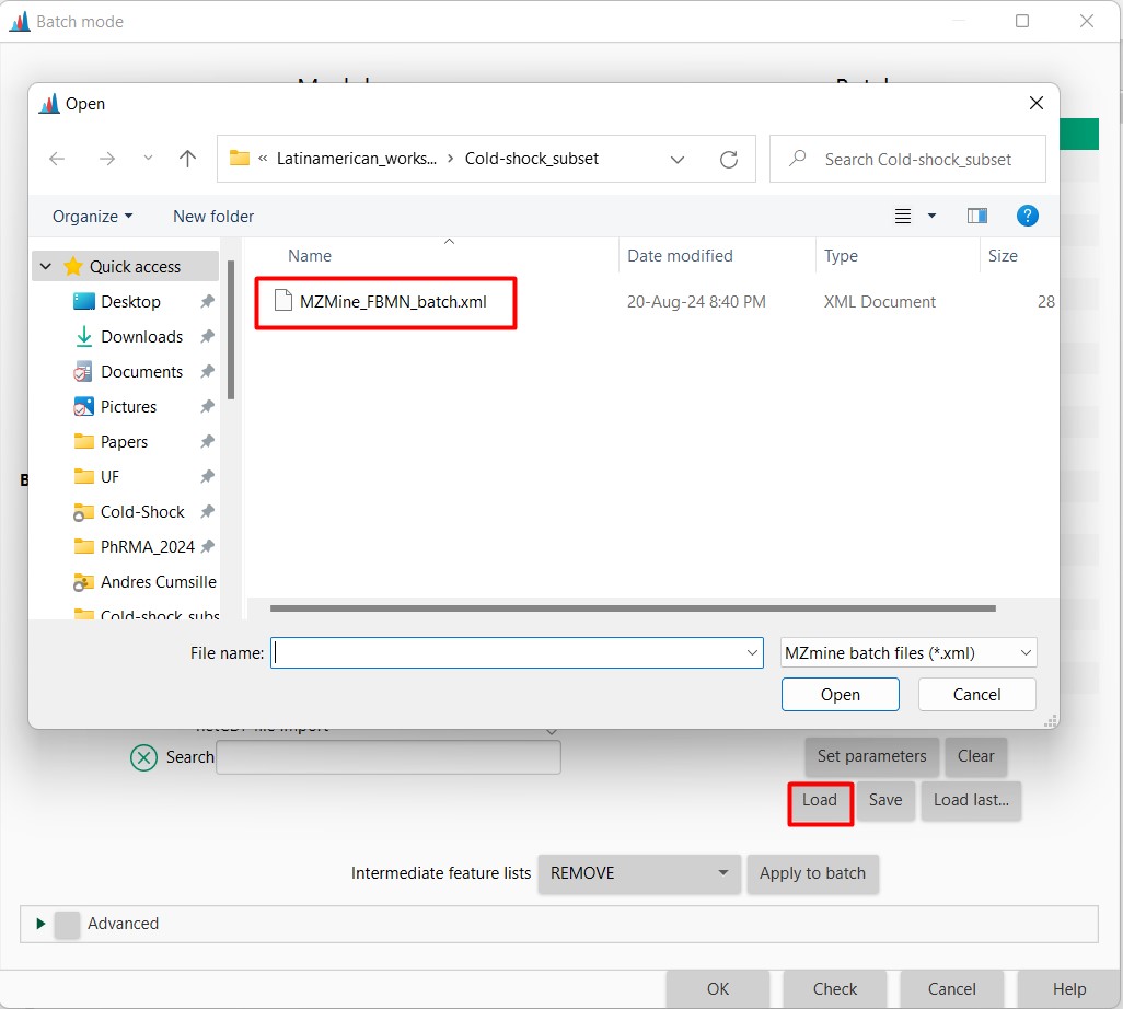
Then double-click on import MS data
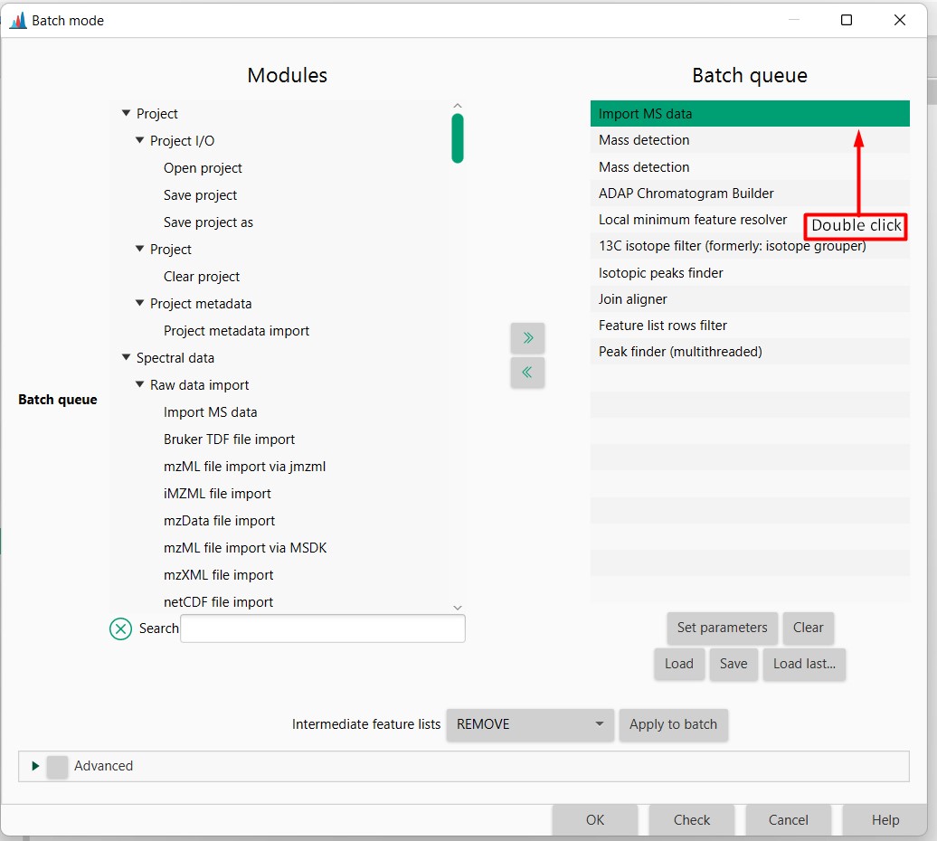
Select from your computer the 18 mzML files from this dataset
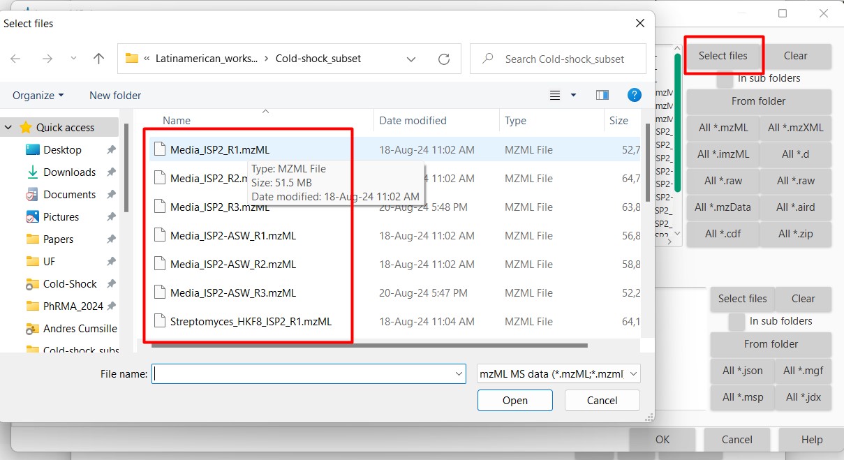
After this, every file should be included in the batch-processing mode. Select OK afterward so the files begin to process in the meantime.
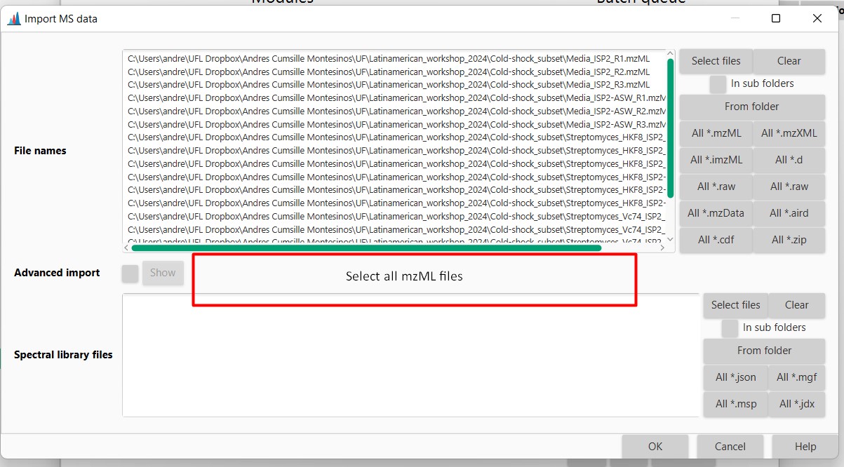
Briefly, MZMine is now detecting all the masses present in your samples, grouping them, and then aligning them, so you can know in which sample each detected spectrum is present
You should note, that the parameters used are specific for this dataset, you might need to change some of the values when analyzing your own samples.
For more information: Nothias, LF., Petras, D., Schmid, R. et al. Feature-based molecular networking in the GNPS analysis environment. Nat Methods 17, 905–908 (2020). https://doi.org/10.1038/s41592-020-0933-6
Explore the structure of our data
In the “MS data files” from MZMine you can observe all the 18 LC-MS/MS files in mzML format that we loaded
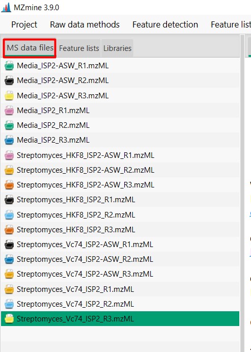
Let’s inspect what the two of these files look like. We could select one file from Streptomyces sp. H-KF8 in ISP2, and one in ISP2-ASW We can select both files, then right-click and select “Show chromatograms”
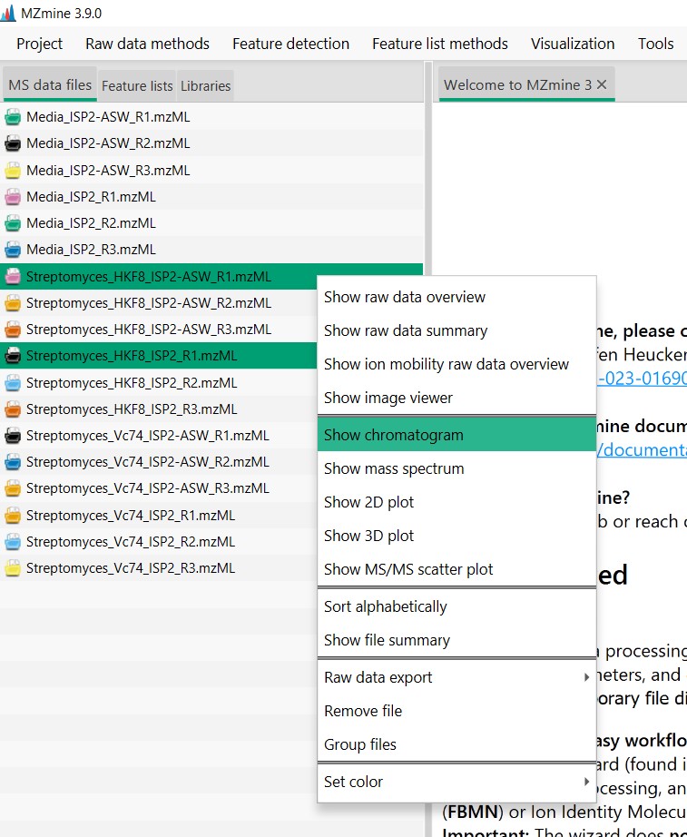
Here we can select the mass range that we want to observe. Since we want to see all the spectra detected, click “Auto range”. It will automatically will select masses ranging from 100 m/z to almost 3,749 m/z Click “OK” then
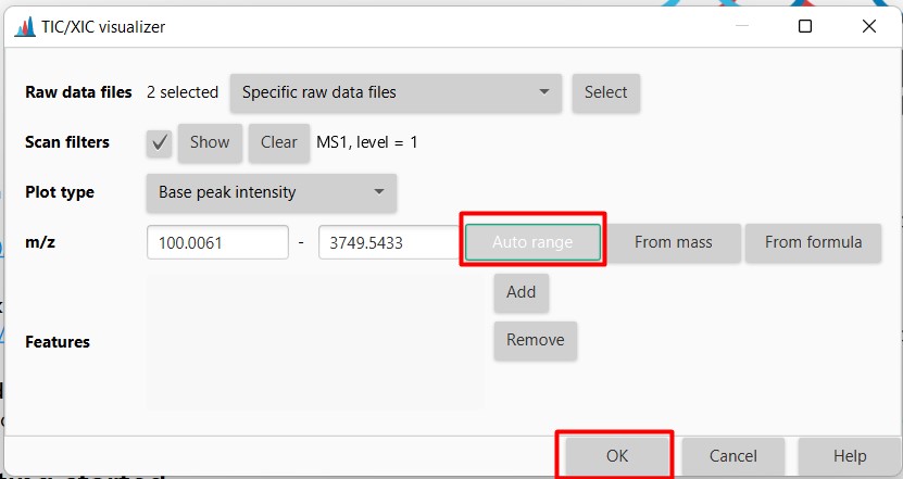
The software will display the Total Ion Chromatogram (TIC) from both samples. In this case, strain H-KF8 is displayed in pink when cultured in ISP2-ASW, and in black when cultured in ISP2
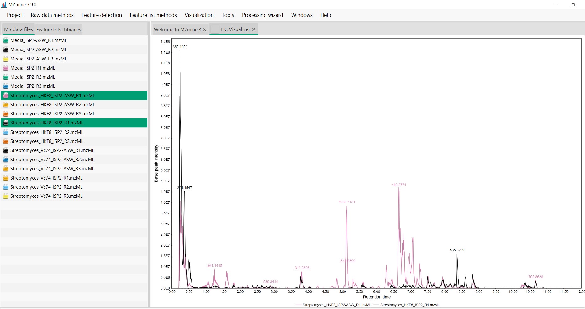
We can select a section of the chromatogram to inspect the differences of the metabolomic profiles of these samples
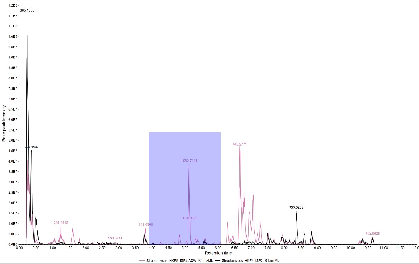
We can observe that several spectra are produced exclusively by strain H-KF8 in ISP2-ASW
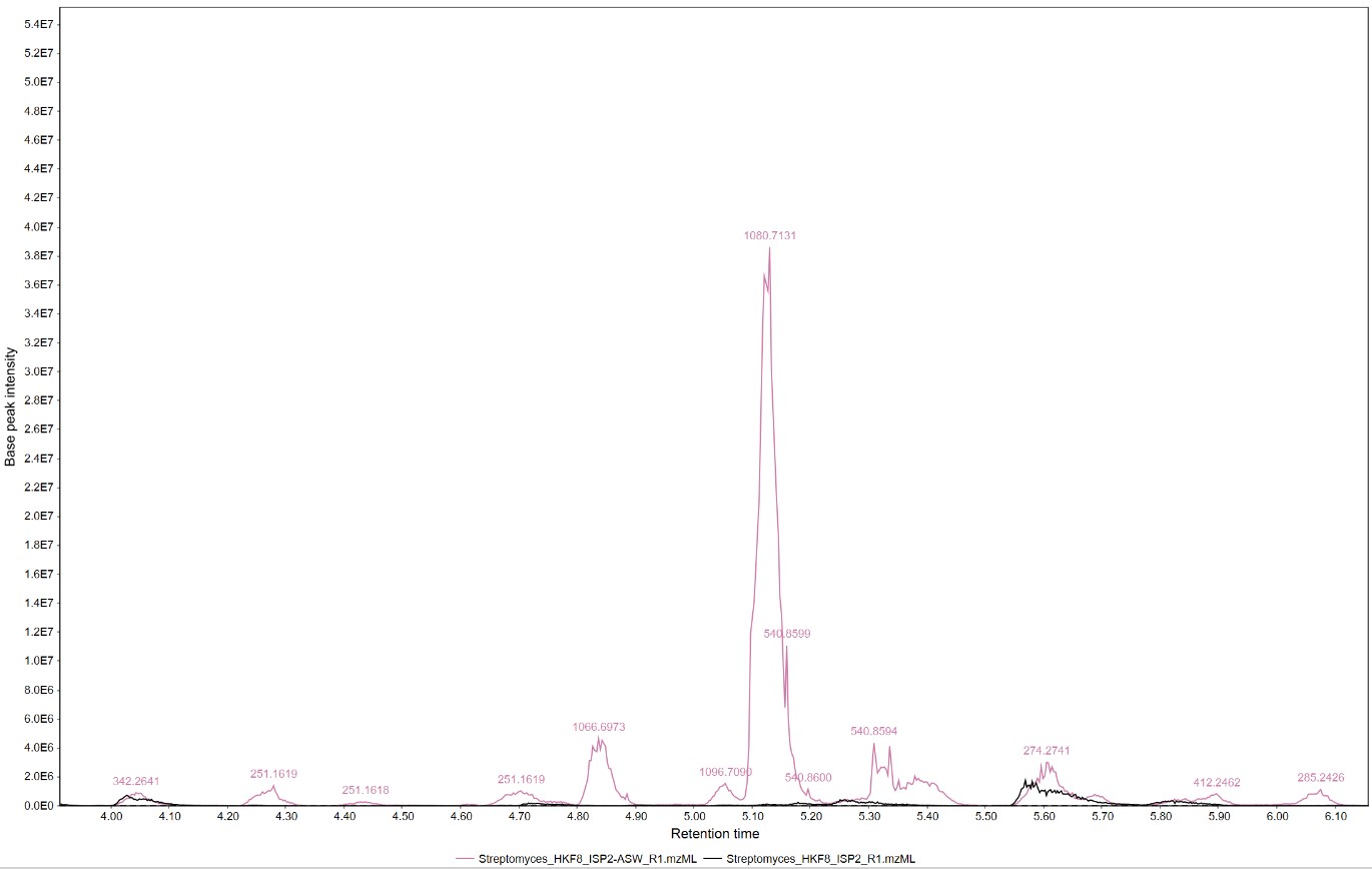
Analyze the final output from the analysis
After processing all files. We should look at the feature lists tab from MZMine. There we can observe that we have a file called “Aligned feature list 13C gaps”. Double-click on that
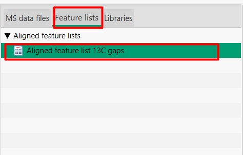
Here we can observe the feature list, where each row is one detected MS spectra with its m/z and retention time (RT). Each column is one of the 18 samples. If MS spectra are detected in a sample, then the height of the peak is displayed in the table
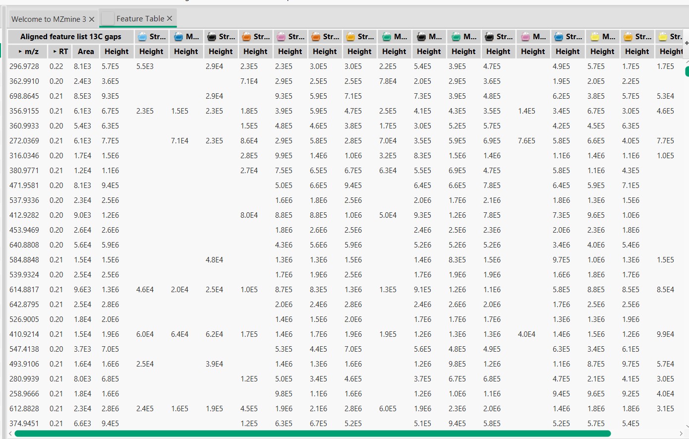
Remove media blanks MS spectra
Now we want to remove all the MS spectra that are part of the culture media and not produced by our strains.
For that, we need to go to “Feature List Methods”, then click on “Feature List Filtering”, and then on “Feature List Blank Subtraction”
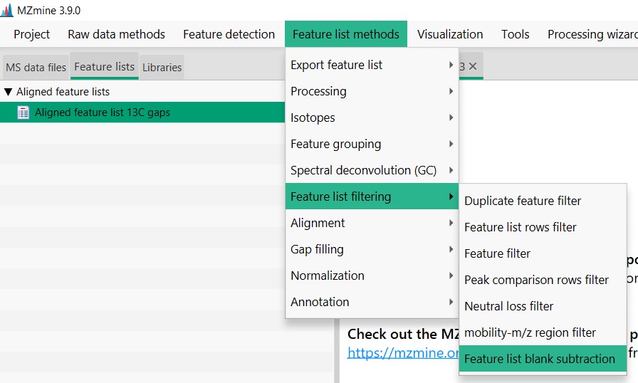
In the “Blank/Control raw data files” section, we need to select “Specific raw data files”, and then select
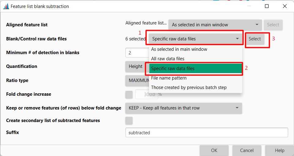
Here we need to select all the samples that belong to the crude extracts from the Media. There are 6 in total. Press OK afterward
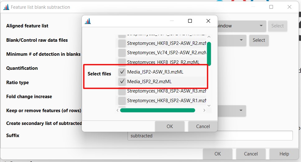
Now we have two Feature lists
- Aligned feature list 13C gaps. That is the original feature list including media MS spectra
- Aligned feature list 13C gaps subtracted. Feature list with media blanks removed
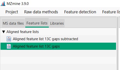
Export Feature lists in GNPS format
We are going to export both Feature lists.
First, select “Aligned feature list 13C gaps”. Then go to “Feature List Methods”, “Export Feature List”, and select Molecular “networking files”
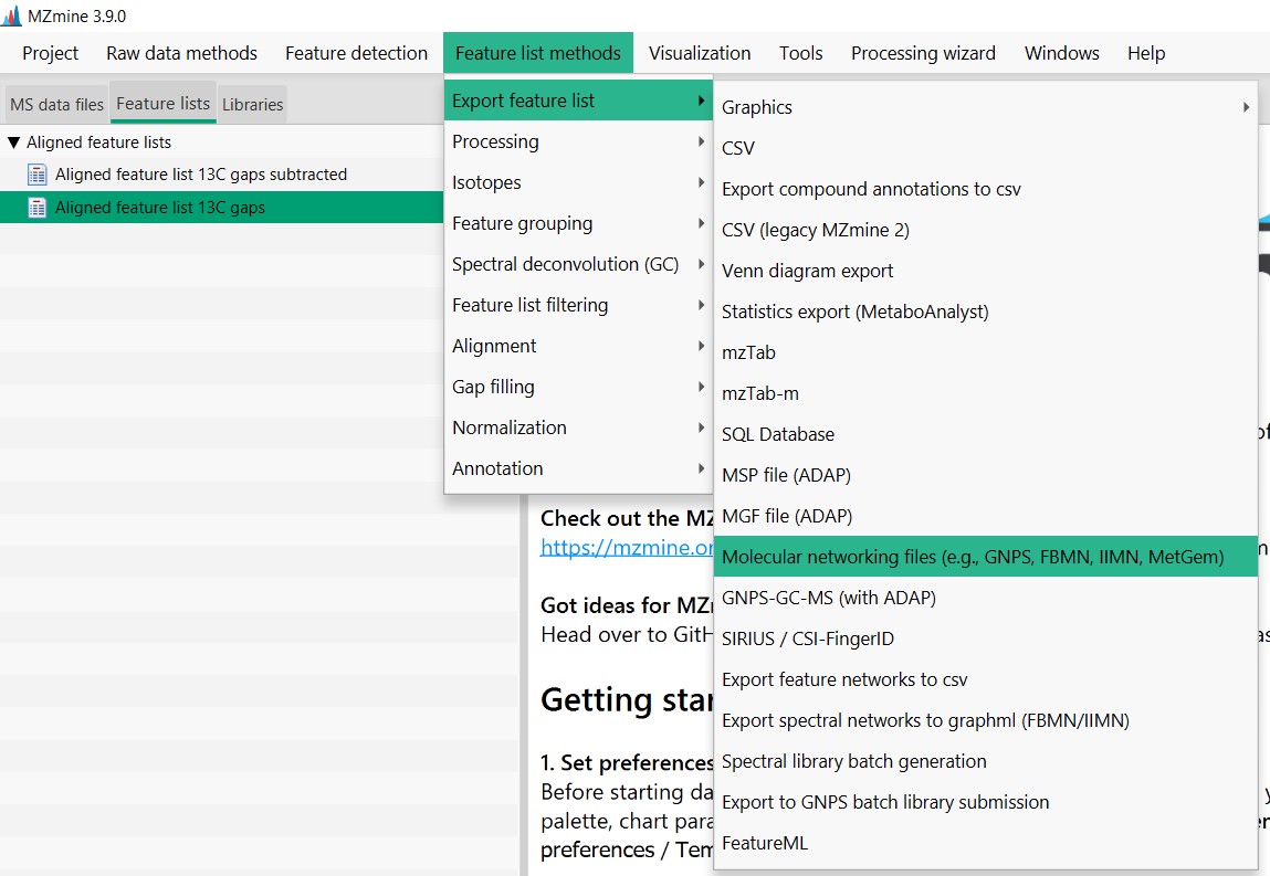
Then click “Select”, and in “File name” write the name that you want your files to be named. In this case, I selected “GM_workshop_Featurelist_complete”. So I know that this file is from the Latin American genome mining workshop and that the feature list includes the media blank MS spectra. then press “save”
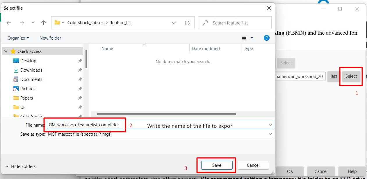
Make sure that in Filter rows you select “MS2 or ION IDENTITY”, so only MS spectra with MS2 are selected.
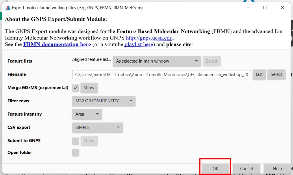
Then, in your selected folder, you should have two files
- GM_workshop_Featurelist_complete_quant.csv
This file is a table that includes all the feature lists in your samples. Again, each row is an MS spectrum, and each column is each of the 18 samples.
- GM_workshop_Featurelist_complete_quant.mgf
This file contains the information on each spectrum. Contains the parent mass in m/z, and the m/z values of each fragment from that spectra, with the peak intensity of each spectrum.
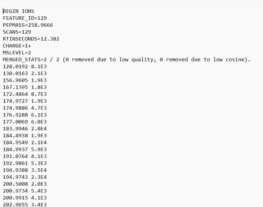
Now we need to repeat the export step but with the media blanks removed. This time the files will be named “GM_workshop_Featurelist_filtered” so we can know that there is no MS spectra that are originally from the culture media.
After this, we have 4 files. And we are done with the processing steps in MZMine 3
Create a molecular network
Go into GNPS webpage
and login using your username and password
Then we should go to “Advanced Analysis Tools”, and Select “Analyze” in the Feature Networking
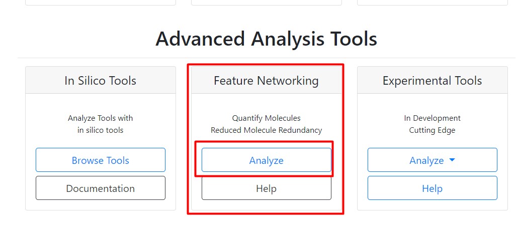
Then we should write a title for our network. We could use something like “GM_workshop_FBMN_filtered”, because we are going to use the feature list with the media blanks removed.
Following that, in “File Selection”, click on “Select Input File”
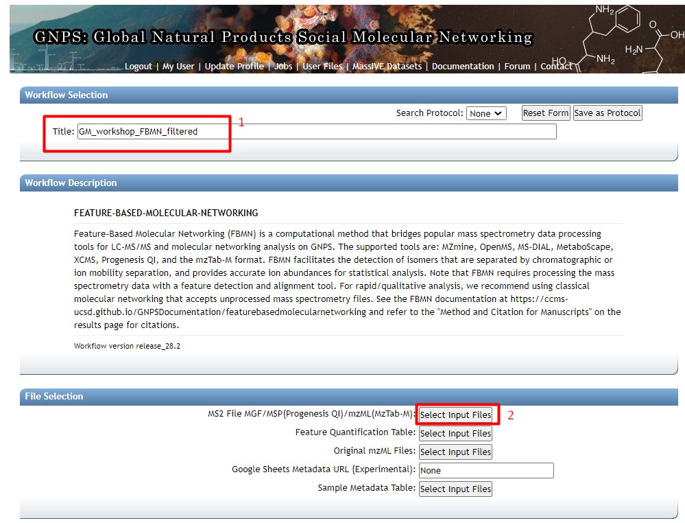
We now need to upload our feature lists and our metadata table. Click on “Upload files”
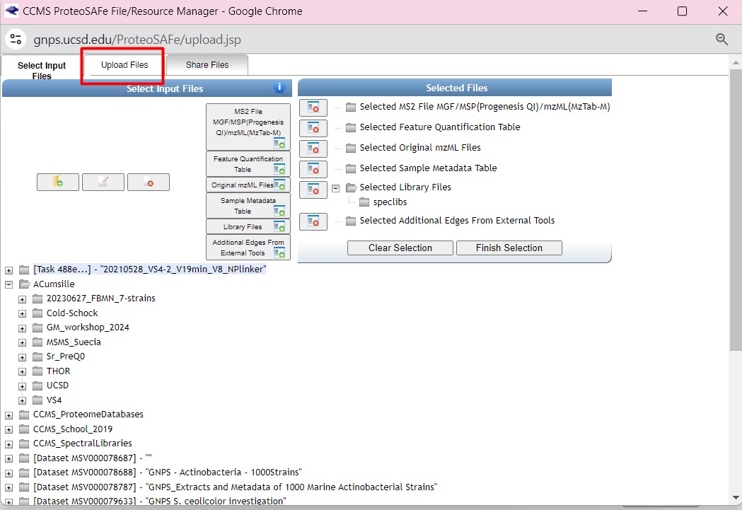
Here we can create a folder in our GNPS. I created a new folder called “LATAM_GM_workshop”. Click on that folder. Then in the “File Drag and Drop”, drag and drop the following files:
- GM_workshop_Featurelist_filtered.mgf
- GM_workshop_Featurelist_filtered_quant.csv
- metadata_table.tsv
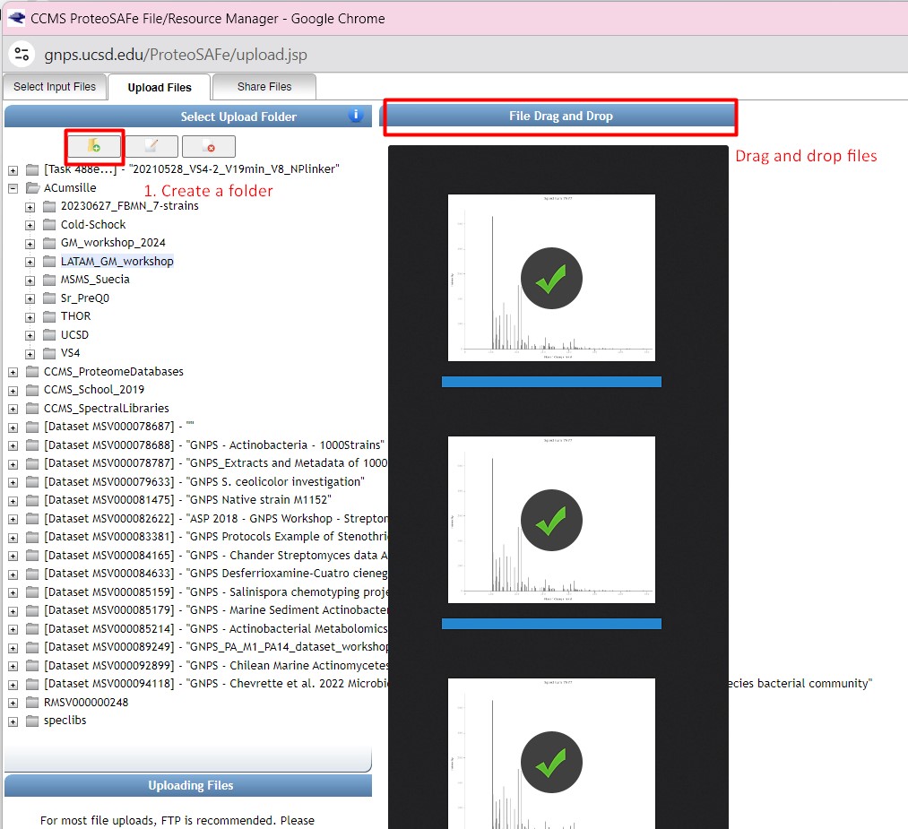
Return to the “Select Input Files” after uploading your files. You should be able to see the three uploaded files in your directory
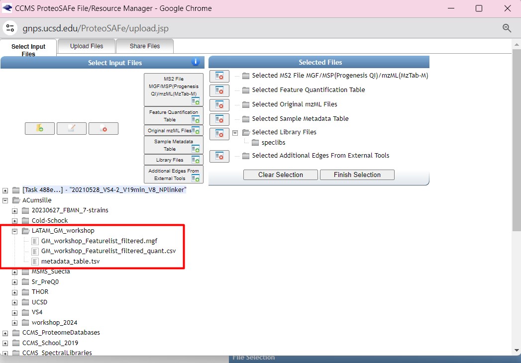
We are going to select the “GM_workshop_Featurelist_filtered.mgf” file as “MS2 file in MGF format”
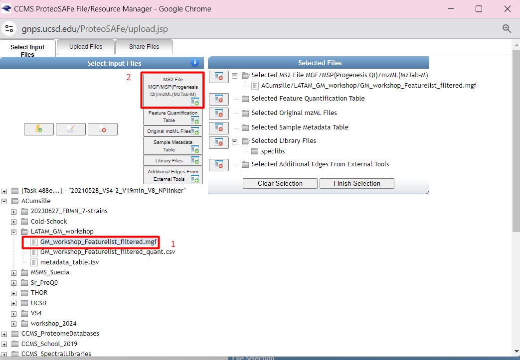
then we are going to select “GM_workshop_Featurelist_filtered_quant.csv” as the “Feature Quantification Table”
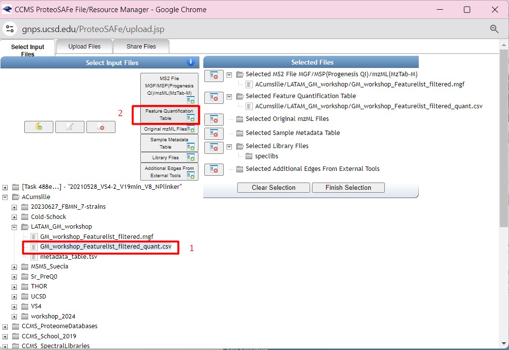
Finally, we are going to select the “metadata_table.tsv” as our “Sample Metadata Table”
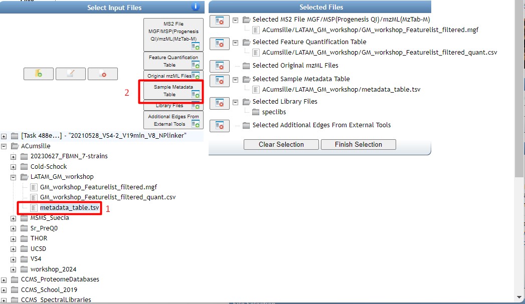
In the “Selected Files” section, we should be able to see the three files in their corresponding sections. Click on finish selection after checking everything is ok.
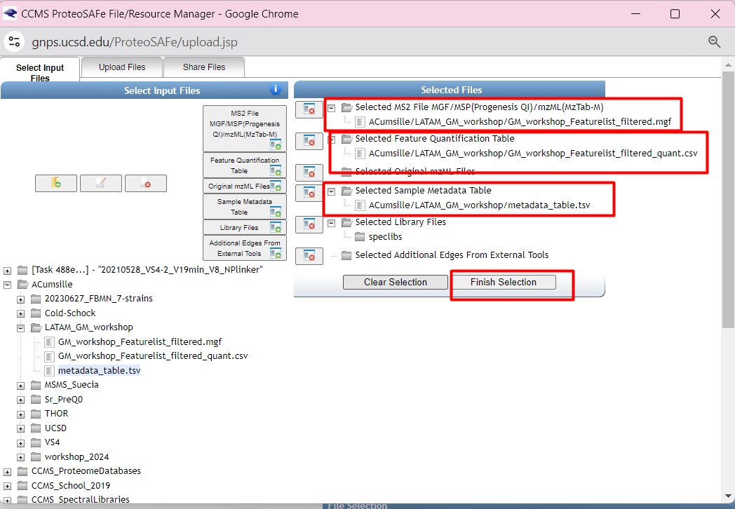
After selecting the files, we need to adjust the parameters for our network Since our data was collected using a high-resolution LC-MS/MS, we could adjust the
- “Precursor Ion Mass Tolerance” to 0.02 Da This value affects the clustering of nearly identical MS/MS spectra through MS-Cluster.
- “Fragment Ion Mass Tolerance” to 0.02 Da Sets the allowable deviation in m/z values for fragment ions when clustering MS/MS spectra
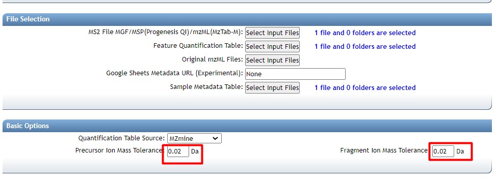
Then we need to select our thresholds to create the molecular network
- “min pair cos” to 0.7 The minimum cosine score required between a pair of consensus MS/MS spectra for an edge to be created in the molecular network.
- “Minimum matched fragment ions” to 6 Specify the minimum number of common fragment ions that two consensus MS/MS spectra must share to be connected by an edge in the molecular network.
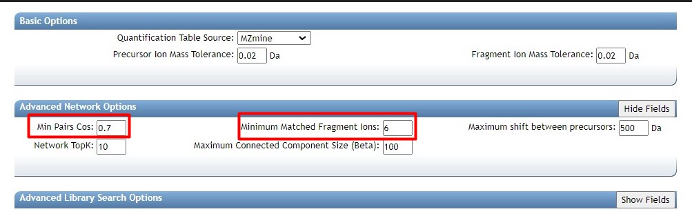
After this, write your email, so you know when your network is finished. Then click “Submit”
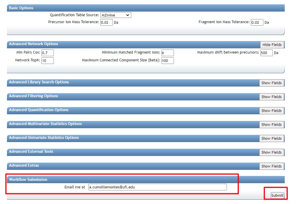
For more information about the rest of the parameters used for molecular networking:
- visit the GNPS documentation
- Also visit Aron, A.T., Gentry, E.C., McPhail, K.L. et al. Reproducible molecular networking of untargeted mass spectrometry data using GNPS. Nat Protoc 15, 1954–1991 (2020).
Statistics analysis using FBMN STATS guide web server
Now we want to observe how different are the metabolic profiles of our samples. For that, we are going to calculate a Principal Coordinate Analysis (PCoA)
Go into FBMN STATS guide
Select “Data Preparation”
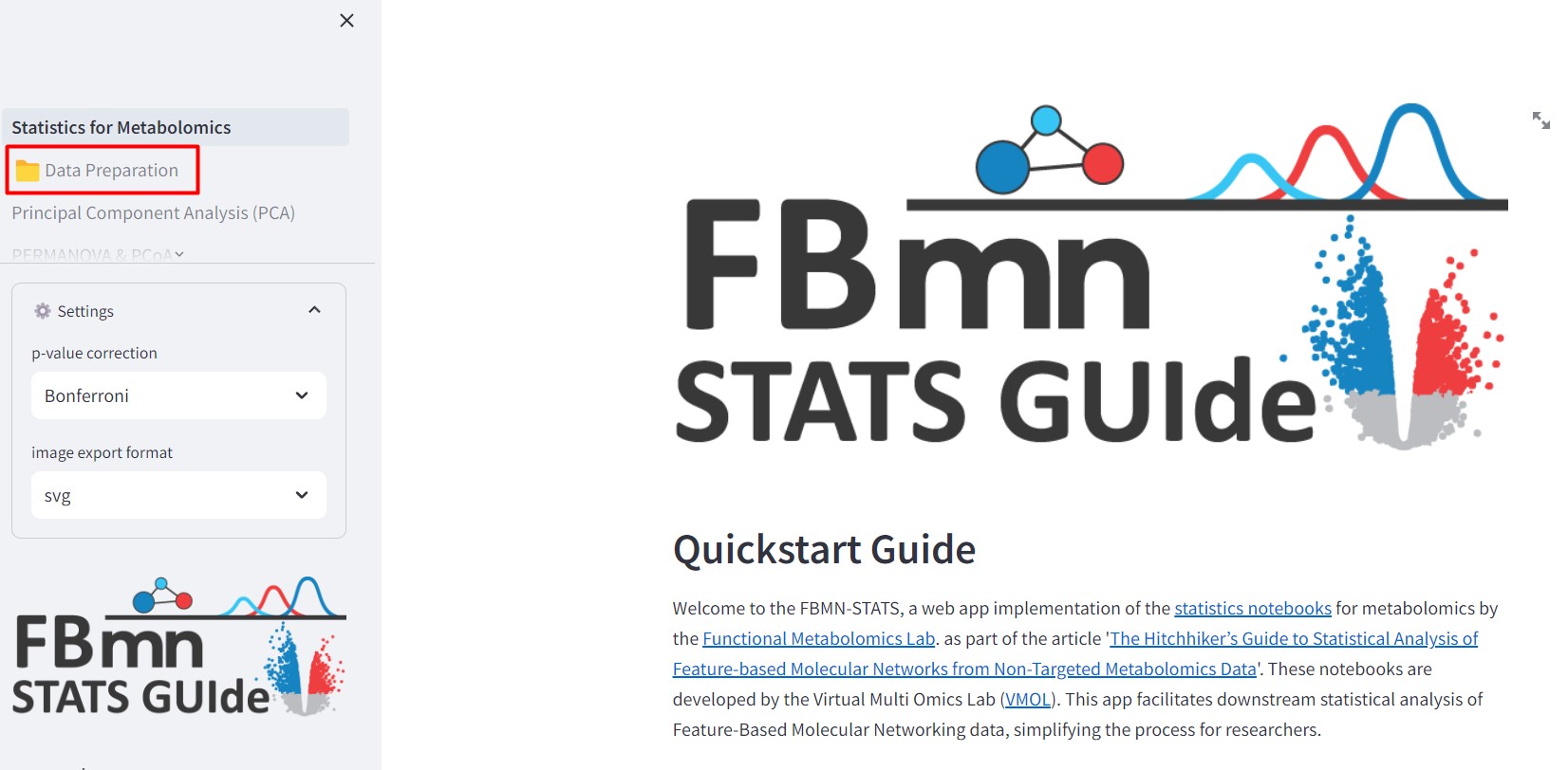
In file origin select “Quantification table and metadata files”.
- In the Quantification Table section, select the MZMine output file “GM_workshop_Featurelist_complete_quant.csv”. This table contains the information of the two strains and the media. We want to observe how different our samples’ metabolomic profiles are, in comparison with the culture media.
- in the Meta Data Table section, include our metadata file “metadata_table.tsv”.
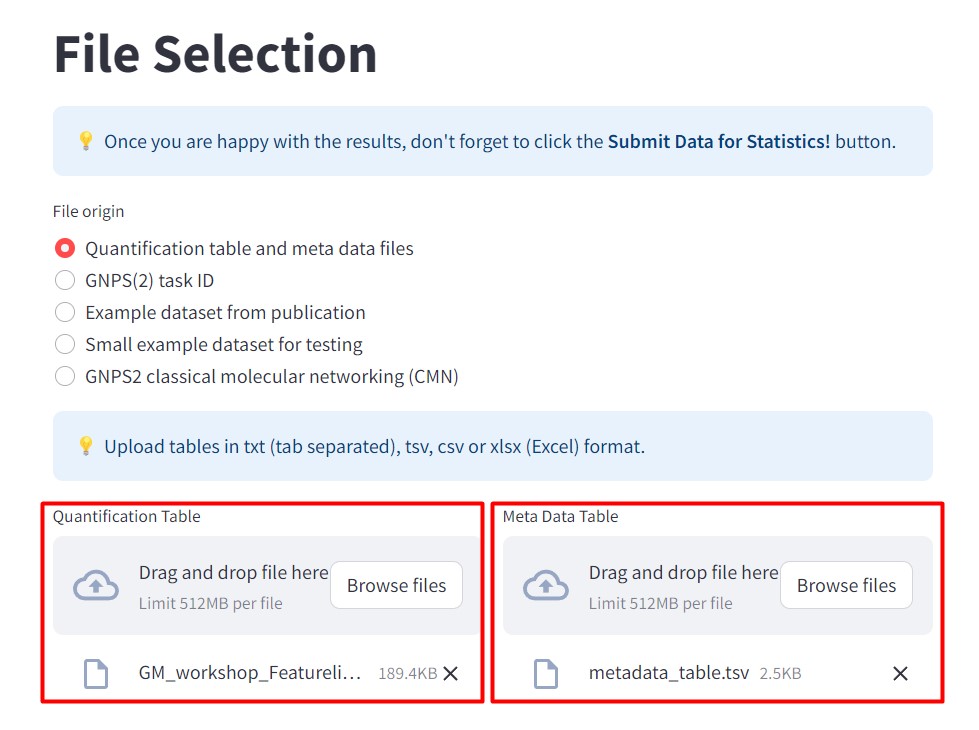
After loading your files, click “Submit Data for Statistics!”.
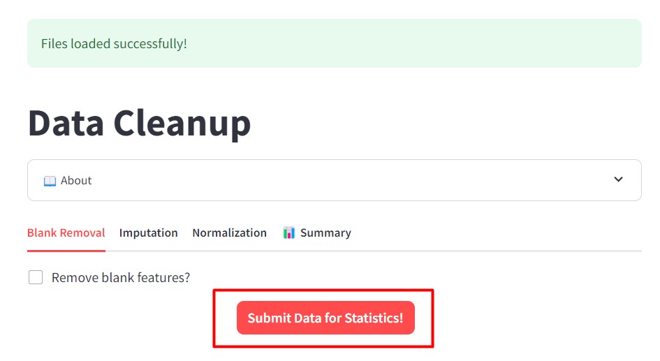
Check that your data have been properly submitted by checking that you have the “Data preparation was successful!”.
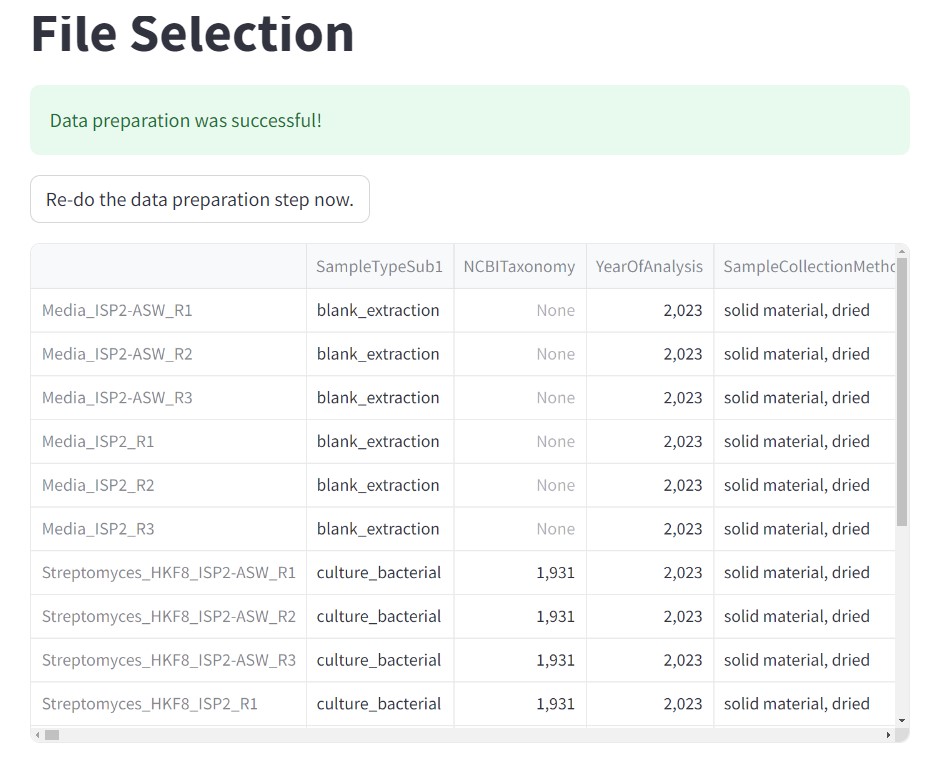
Now we should go to the “PERMANOVA & PCoA” section.
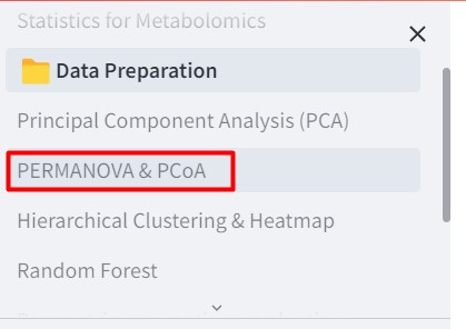
Select Principal Coordinate Analysis.
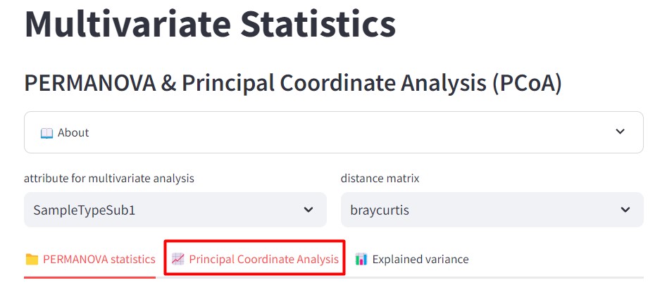
Now we could change how we want to color our samples. Select “attribute for multivariate analysis” ATTRIBUTE_media. This will color our samples according to the media (ISP2 or ISP2-ASW)
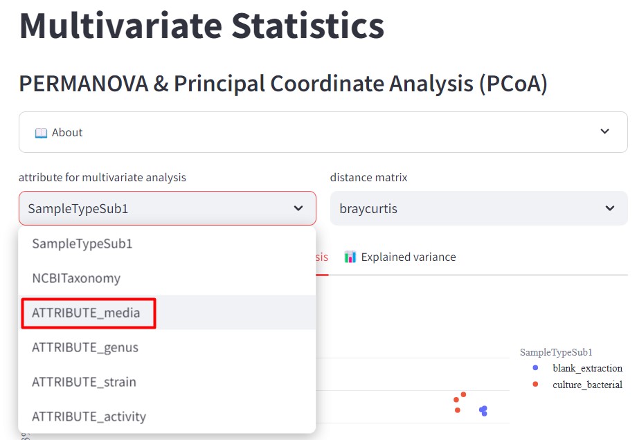
We can observe that there is a difference between the samples prepared with ISP2 and ISP2-ASW
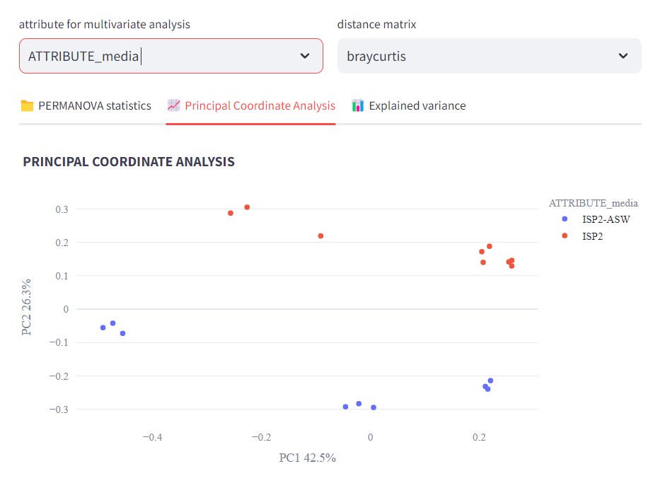
Now if we color our samples by strain, selecting ATTRIBUTE_strain in “attribute for multivariate analysis”
We can observe that Streptomyces sp. Vc74B-19 metabolic profile is quite different than the ones from Streptomyces sp. H-KF8 and the culture media.
Also, it is possible to observe that Streptomyces sp. H-KF8 metabolomic profile differs more from the media when cultured in ISP2-ASW
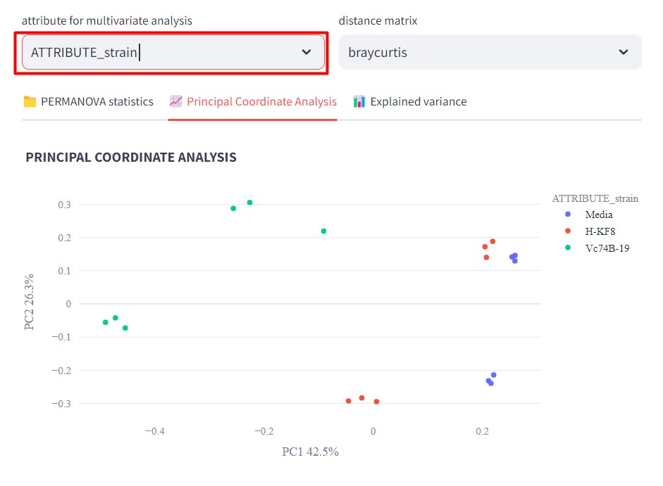
There are several statistics that you can do using FBMN STATS guide, you can check the preprint here.
Visualize the network using Cytoscape
We need to check if our GNPS network is done processing. You might have received an email, otherwise, go to your GNPS account and click on “Jobs”
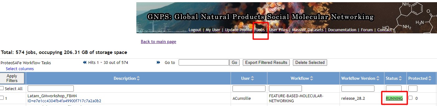
If your network is Done, then click on it. Afterward, click on “Direct Cytoscape Preview/Download”
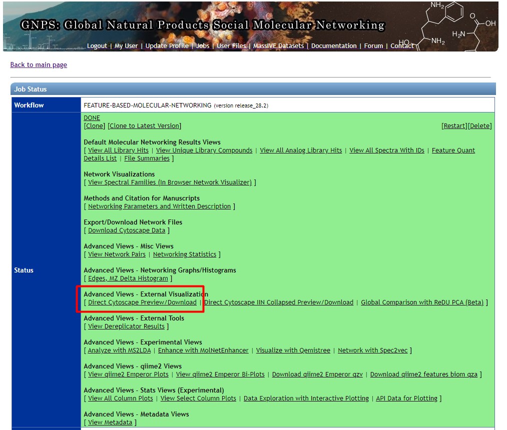
If your network is not Done, then we could use a previously computed network, that holds the same data that we used in this workshop
Click on “Download Cytoscape File”, and save it in your computer
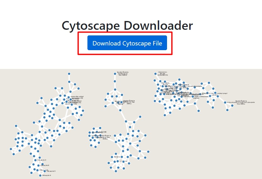
Open the network on Cytoscape. We want to change the style of the network and color the nodes according to the strains. Click on “Style”
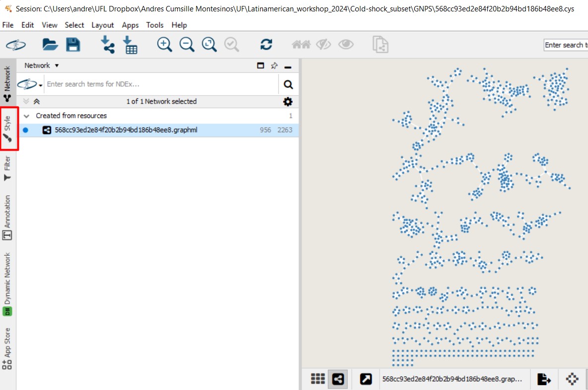
Select the pie chart icon on Image/Chart. This will help us figure out the abundance of each MS spectra, depending on the metadata parameter that we choose
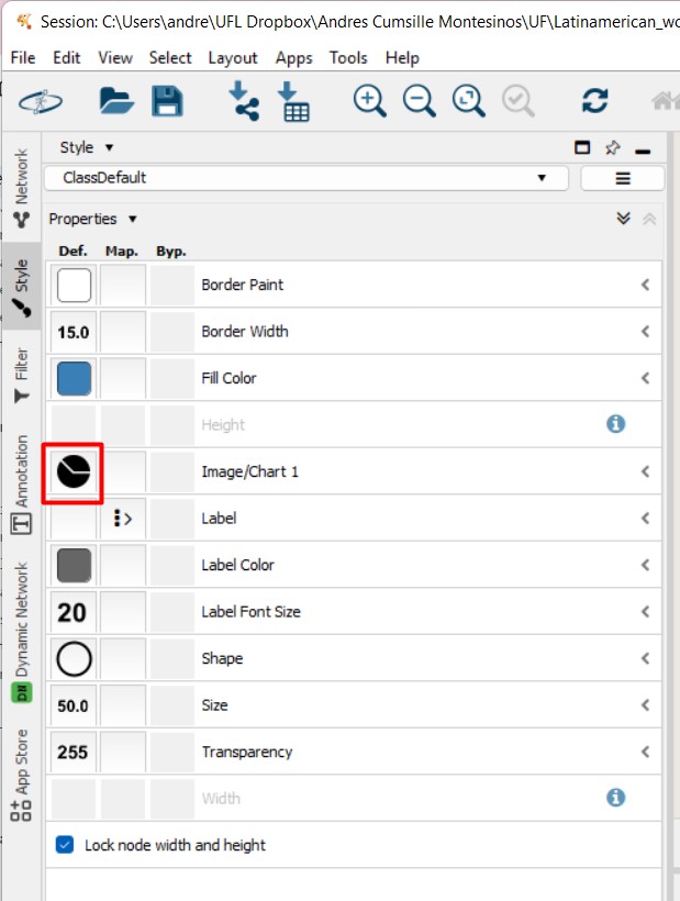
In this case, we will select the two strains, and also the media Although we removed all the MS spectra present in the media, there might still be some nodes with MS spectra detected in some of the media samples.
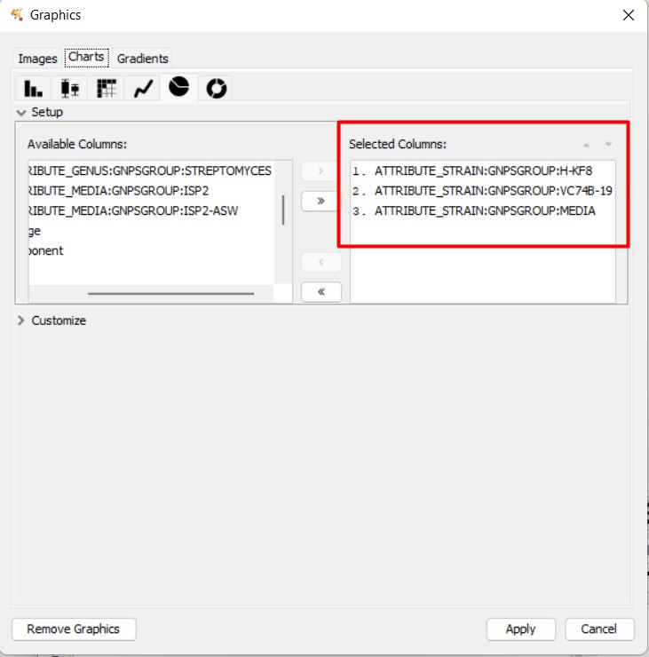
If we click “Apply”, we can observe the nodes present in each strain, and the media. In this case, the light blue means the MS spectra detected in Streptomyces sp. Vc74B-19
In this Molecular Family, we can observe some MS spectra with annotations. Some are similar to Urdamycinone B, Dehydroxyaquayamycin, and other Angucycline-related compounds.
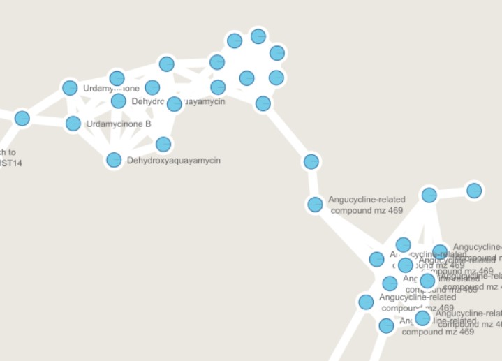
We can color now the nodes depending on the media where they are detected. Select the pie chart again in “Image/Chart”, and now select ISP2 and ISP2-ASW. This will color ISP2 in red, and ISP2-ASW in light blue
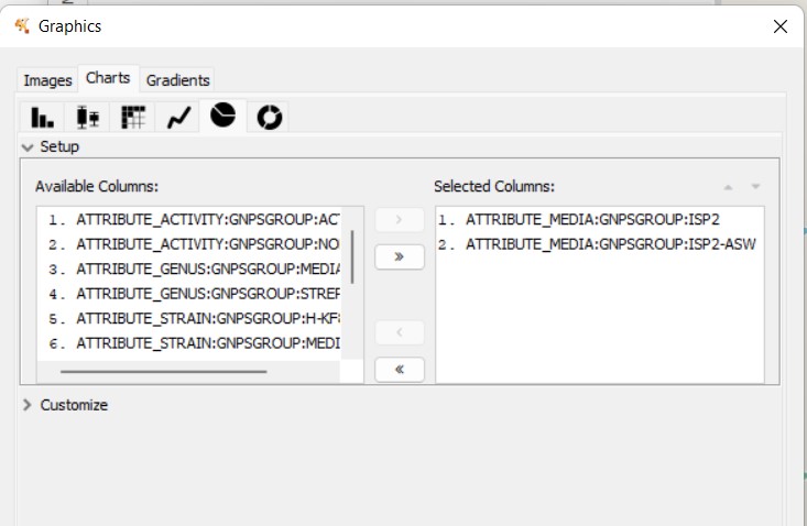
We can observe that some nodes are detected mostly in ISP2. However, several angucycline-related compounds are detected almost exclusively in ISP2-ASW
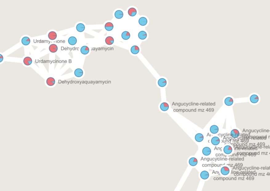
References
- Wang, M., Carver, J., Phelan, V. et al. Sharing and community curation of mass spectrometry data with Global Natural Products Social Molecular Networking. Nat Biotechnol 34, 828–837 (2016). https://doi.org/10.1038/nbt.3597.
- Schmid, R., Heuckeroth, S., Korf, A. et al. Integrative analysis of multimodal mass spectrometry data in MZmine 3. Nat Biotechnol 41, 447–449 (2023). https://doi.org/10.1038/s41587-023-01690-2.
- Nothias, LF., Petras, D., Schmid, R. et al. Feature-based molecular networking in the GNPS analysis environment. Nat Methods 17, 905–908 (2020). https://doi.org/10.1038/s41592-020-0933-6
- Aron, A.T., Gentry, E.C., McPhail, K.L. et al. Reproducible molecular networking of untargeted mass spectrometry data using GNPS. Nat Protoc 15, 1954–1991 (2020). https://doi.org/10.1038/s41596-020-0317-5
- Shah, A. K. P., Walter, A., Ottosson, F., Russo, F., Navarro-Díaz, M., Boldt, J., Kalinski, J.-C., Kontou, E. E., Elofson, J., Polyzois, A., González-Marín, C., Farrell, S., Aggerbeck, M. R., Pruksatrakul, T., Chan, N., Wang, Y., Pöchhacker, M., Brungs, C., Cámara, B., … Petras, D. (2023). The Hitchhiker’s Guide to Statistical Analysis of Feature-based Molecular Networks from Non-Targeted Metabolomics Data. ChemRxiv, 1–83. https://doi.org/10.26434/CHEMRXIV-2023-WWBT0
In the future it will include:
- https://www.tfleao.com/general-8,
- Paired omics
- In the future it will include: SIRIUS: Kai Dührkop, Markus Fleischauer, Marcus Ludwig, Alexander A. Aksenov, Alexey V. Melnik, Marvin Meusel, Pieter C. Dorrestein, Juho Rousu, and Sebastian Böcker, SIRIUS 4: Turning tandem mass spectra into metabolite structure information. Nature Methods 16, 299–302, 2019.
- Data is generated using Liquid Chromatography coupled to a tandem mass spectrometer (LC-MS/MS or MS2).
- Dereplication is the process of identifying previously known compounds.
- Molecular networking is a computational method that organizes MS2 data based on spectral similarity, allowing us to infer relationships between chemical structures
- Feature-Based Molecular Networking (FBMN) enhances classical molecular networking by integrating relative quantitative data, enabling more robust metabolomics statistical analysis.
Content from Other Resources
Last updated on 2026-02-20 | Edit this page
Estimated time: 20 minutes
Overview
Questions
- What else can I do?
Objectives
- First learning objective. (FIXME)
Other resources
We have seen how to conduct a genome mining project with some particular characteristics. However, each research project may need some deviations to these workflows. You may need to make use of RNA-Seq data to search just for some specific domains instead of complete BGCs or to combine metabolomics or proteomics with genomic data. Here we will provide a list of resources that are also useful for genome mining projects.
Assemblers
First, since BGCs usually encompass genes with high levels of repeat regions (mainly NRPSs and PKSs), genome assemblers are not always capable of reconstructing BGCs and sometimes divide them into two contigs. To overcome this difficulty, you can use biosyntheticSPADes to assemble your reads into complete BGCs. This algorithm is implemented within the SPAdes tool.
Other genome mining programs
Depending on your interests, you can use some alternative program to search for BGCs in your genomes. The Secondary Metabolite Bioinformatics Portal lists and introduces many diverse bioinformatic tools that pursue this goal. For example, CLUSEAN and NaPDoS allow to detect PKS and NRPS domains, while BAGEL, RODEO and RiPPMiner are dedicated to find ribosomally synthesized and post-translationally modified peptides (RIPPs). Then, implementing a further step, ARTS prioritizes previously detected BGCs (with antiSMASH) and identifies drug targets from these data.
There are also some tools and workflows that are dedicated to finding new biosynthetic systems (new types of BGCs or biosynthetic genes). Among them, as it was explained in previous lessons, EvoMining arose as a promising tool to detect biosynthetic enzymes that may have evolved from developing core functions (‘central’ or ‘primary’ metabolism) to carry on specialized functions (secondary metabolism). Likewise, ClusterFinder enables the prediction of uncharacterized BGCs in genomes through different algorithms.
Tools for metabolomics
You can also try to link diverse -omics data with genome predictions. SeMa-Trap allows the use RNA-Seq data to find co-expression patterns between certain genes and BGCs. Similarly, if you need to combine metabolomic/proteomic data with putative BGCs-products, you can use Pep2Path, MetaMiner or GNPS, amongst others.
Phylogeny based tools
Finally, to prioritize genomes or species, autoMLST allows you not only to find phylogenetically closed strains/species from your input genome but also to explore the biosynthetic potential of those relatives.
Specialized data bases
- BGCs in human Microbiome Humi
Carpentries Philosophy
A good lesson should be as complete and transparent as easy to teach by any instructor. Carpentries lessons are developed for the community; now, you are part of us. This lesson is being developed, and we are sure that you can collaborate and help us improve it.
- First key point. Brief Answer to questions. (FIXME)