Content from Introduction
Last updated on 2026-02-12 | Edit this page
Overview
Questions
- What is machine learning?
Objectives
- Define and give examples of machine learning
- Identify problems in computational biology suitable for machine learning
What is this workshop about?
The learning objectives of this workshop are:
Identity and characterize machine learning and a machine learning workflow.
Evaluate whether a particular problem is easy or hard for machine learning to solve.
Assess a typical machine learning methodology presented in an academic paper.
Gain confidence in and appreciation for machine learning in biology.
We will also be learning about some specific machine learning models: decision trees, random forests, logistic regression, and artificial neural networks.
What is machine learning?
Definition
Machine learning is a set of methods that can automatically detect patterns in data and then use those patterns to make predictions on future data or perform other kinds of decision making under uncertainty.
A machine learning algorithm gets better at its task when it is shown examples as it tries to define general patterns from the examples.
One of the most popular textbooks on machine learning, Machine Learning by Tom Mitchell, defines machine learning as, “the study of computer algorithms that improve automatically through experience.”
Definition
Algorithm - is a relationship between input and output. It is a set of steps that takes an input and produces an output.
Machine learning can be broadly split into two categories, supervised machine learning and and unsupervised learning. Machine learning is considered supervised when there is a specific answer the model is trying to predict, questions like what is the price of a house? Is this mushroom edible? What disease does this patient have? Some examples of supervised machine learning are classification and regression. These will be further defined in the next lesson.
Unsupervised machine learning has no particular target for its learning, it is instead trying to answer general questions about patterns. This can include questions like how do these cells group together? In what way are these samples most different from each other? An example of unsupervised machine learning is clustering. Unsupervised learning will not be covered in this workshop. For some external resources, check out the [references][lesson-reference].
Definitions
Supervised learning - training a model from the labeled input data.
Unsupervised learning - training a model from the unlabeled input data to find patterns in the data.

Definition
Clustering - grouping related samples in the data set.
Classification - predicting a category for the samples in the data set.
Regression - predicting a continuous number for the samples in the data set.
Classifier - a specific model or algorithm that performs classification.
Model - mathematical representation that generates predictions based on the input data.
Scenarios
Consider whether the following 3 scenarios should or should not be considered machine learning.
You are trying to understand how temperature affects the speed of embryo development in mice. After running an experiment where you record developmental milestones in mice at various temperatures, you run a linear regression on the results to see what the overall trend is. You use the regression results to predict how long certain developmental milestones will take at temperatures you’ve not tested.
You want to create a guide for which statistical test should be used in biological experiments. You hand-write a decision tree based on your own knowledge of statistical tests. You create an electronic version of the decision tree which takes in features of an experiment and outputs a recommended statistical test.
You are annoyed when your phone rings out loud, and decide to try to teach it to only use silent mode. Whenever it rings, you throw the phone at the floor. Eventually, it stops ringing. “It has learned. This is machine learning,” you think to yourself.

What is the difference between a machine learning algorithm and a traditional algorithm?
Traditional algorithm: Let’s say you are doing an experiment, and you need to mix up some solutions. You have all the ingredients, you have the “recipe” or the proportions, and you follow the recipe to get a solution.
Machine learning algorithm: You are given the ingredients and the final solution, but you don’t know the recipe. So, what you need to do it to find the “fitting” of the ingredients, that would result in your solution.
Think about the following questions whenever we encounter a situation involving machine learning.
What does machine learning mean for biology?
Machine learning can scale, easily making predictions on a large number of items. It can be very slow and expensive for expert biologists to manually make the same decisions or manually construct a decision-making model. Training and executing a machine learning model can be faster and cheaper. Machine learning may also recognize complex patterns that are not obvious to experts.
Let’s look at some examples of how machine learning is being used in biology research.
- Imputing missing SNP data.
- Identifying transcription-factor binding sites from DNA sequence data alone, and predicting gene function from sequence and expression data.
- Finding drug targets in breast, pancreatic and ovarian cancer.
- Diagnosing cancer from DNA methylation data.
- Finding glaucoma in color fundus photographs using deep learning.
- Predicting lymphocyte fate from cell imaging
- Predicting 3d protein structures
- Discovering new antibiotics
- Recognizing clinical impact of genetic variants
A guide to machine learning for biologists is an excellent reference that covers many of the concepts discussed in this workshop.
- Machine learning algorithms recognize patterns from example data
- Supervised learning involves predicting labels from features
Content from Classifying T-cells
Last updated on 2026-02-12 | Edit this page
Overview
Questions
- What are the steps in a machine learning workflow?
Objectives
- Define classifiers
- Identify the parts of a machine learning workflow using machine learning terminology
- Summarize the stages of a machine learning workflow
- Describe how training, validation, and test sets can avoid data leakage
Why classify T-cells
Consider how to answer a biological question using machine learning. The question pertains to immunotherapy, a type of cancer treatment that uses the body’s immune cells to attack cancer. T-cells are a common target for immunotherapies. For immunotherapy to be effective, the modified T-cells must be in an active state. Here we will study how to assess the activation state of individual T-cells.
Scientists at UW-Madison and the Morgridge Institute developed an imaging method to quickly acquire images of T-cells without destroying them. These images contain information that can be used to predict T-cell activity. The goal is to develop a classifier that can take an image of a T-cell and predict whether it is active or quiescent. The active cells would then be used for immunotherapy, and the quiescent cells can be considered inactive and would be discarded.
Definitions
Active cells - Cells that have become active in their functions. For T-cells, this means increased cell growth and differentiation, typically after being activated by an antigen.
Quiescent cells - Cells that are in an inactive state.
Dataset description
This microscopy dataset includes grayscale images of two type of T-cells: activated and quiescent. These T-cells come from blood samples from six human donors.
| Activated T-cell examples | Quiescent T-cell examples |
|---|---|
 |
 |
 |
 |
 |
 |
We will use a subset of the images and follow the workflow in a T-cell classification study.
Machine learning methods
The goal of this study is to develop a method to classify T-cell activation state (activated vs. quiescent).
Machine learning workflow

Before we can use a model to predict T-cell states, we have to do three steps:
- Preprocessing: Gather data and get it ready for use in the machine learning model.
- Learning/Training: Choose a machine learning model and train it on the data.
- Evaluation: Measure how well the model performed. Can we trust the predictions of the trained model?
Data preprocessing
The first step in machine learning is to prepare our data. Preprocessing the raw data is an essential step to have quality data for the model.
Definitions
Preprocessing - Anything done to a raw dataset before being used for analysis. This can include transformations, format changes, de-noising, removal of poor-quality data, or adding in data that is missing.
Missing values - Parts of a dataset that are not measured or reported. Missing values can be imputed, using statistics to guess their value, or removed.
Outliers - Parts of a dataset that are significantly different from the rest. Outliers can be caused by a true phenomenon or experimental error, in which case they may be removed or transformed to fit the rest of the dataset.
Data normalization - Transforming a feature or set of features of a dataset so they have a certain set of properties. An example would be changing a feature so that all of its values are between 0 and 1, or changing its variance to be 1.
Preprocessing data can include imputing missing values, checking the consistency of the data’s features, choosing how to deal with any outliers, removing duplicate values, and converting all features into a format that is usable by a machine learning algorithm. There are a variety of methods and tools for data normalization and preprocessing.
However, learning these methods and tools is outside the scope of this workshop. Preprocessing strategies are specific to both a dataset’s domain and the technology used to gather the data. Throughout this workshop, we will assume that all of the data has already been preprocessed.
In the T-cell study, preprocessing steps included removing images of red blood cells from the dataset, padding images with black borders to make them all the same size, and extracting cell features with Cell Profiler.
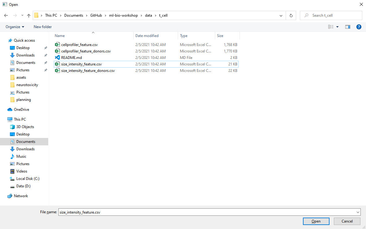
Step 1: Select data
Software
Load t_cell/size_intensity_feature.csv into the ml4bio
software under the Labeled Data by clicking on Select
File…. Note that some of the screenshots below show different
datasets being used.
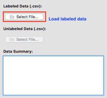
After a valid labeled dataset is loaded, the file name will be shown next to Select File….
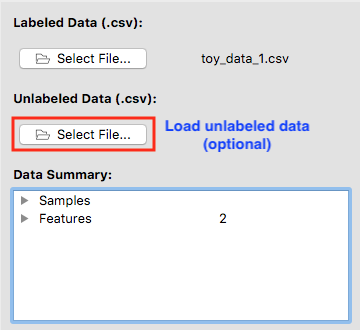
Data summary
Data Summary gives us an insight into features, samples, and class for the dataset we selected.
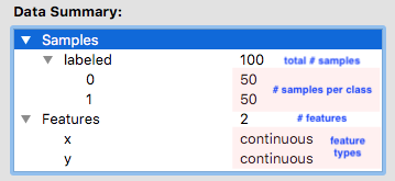
Definitions
Sample - A specific observation in a dataset. In the T-cells example each T-cell is a sample. Also called instances or observations.
Class - The part of a dataset that is being predicted. In the T-cells example a T-cell’s state as active or quiescent is its class. Also called the target variable or label.
Feature - a property or a characteristic of the observed object. Used as an input.
Class label - prediction output. Also called the target variable or label.
In this particular dataset, we can see that we have two features cell_size and total_intensity. The total number of samples is 843.
Questions to consider
How many quiescent samples are in the dataset?
How many active samples?
Can we make any assumptions about the dataset based on the number of samples for each label?
Training set vs. Validation set vs. Test set
Before we continue, split the dataset into a training set and a test set. The training set is further divided into a training set and a validation set.

Definitions
Training set - The training set is a part of the original dataset that trains or fits the model. This is the data that the model uses to learn patterns and set the model parameters.
Validation set - Part of the training set is used to validate that the fitted model works on new data. This is not the final evaluation of the model. This step is used to change hyperparameters and then train the model again.
Test set - The test set checks how well we expect the model to work on new data in the future. The test set is used in the final phase of the workflow, and it evaluates the final model. It can only be used one time, and the model cannot be adjusted after using it.
Parameters - These are the aspects of a machine learning model that are learned from the training data. The parameters define the prediction rules of the trained model.
Hyperparameters - These are the user-specified settings of a machine learning model. Each machine learning method has different hyperparameters, and they control various trade-offs which change how the model learns. Hyperparameters control parts of a machine learning method such as how much emphasis the method should place on being perfectly correct versus becoming overly complex, how fast the method should learn, the type of mathematical model the method should use for learning, and more.
Setting a test set aside from the training and validation sets from the beginning, and only using it once for a final evaluation, is very important to be able to properly evaluate how well a machine learning algorithm learned. If this data leakage occurs it contaminates the evaluation, making the evaluation not accurately reflect how well the model actually performs. Letting the machine learning method learn from the test set can be seen as giving a student the answers to an exam; once a student sees any exam answers, their exam score will no longer reflect their true understanding of the material.
In other words, improper data splitting and data leakage means that we will not know if our model works or not.
Definitions
Data leakage - A model being influenced by data outside the training and validation sets. Data leakage can result in incorrectly estimating how well that model is performing.
Scenarios - Poll
In the following excerpts, consider the methodology presented and determine if there is evidence of data leakage:
We created a decision tree model to predict whether a compound would inhibit cell growth. We trained the model on the 48 available instances, and found that the decision tree was able to predict 96 percent of those instances correctly. Thus, the decision tree is high performing on this task.
We trained 36 different models, each using a different combination of hyperparameters. We trained each model on 80% of the data, withholding 20% of the data to test each model. We present the highest performing model to show the effectiveness of machine learning on this task.
We split the data into training and testing sets of 80% and 20%, and further split the training set into a training and validation set. We trained 200 models on the training data, and chose the best-performing model based on performance on the validation set. After choosing and training the model, we found that the model was able to predict correctly 93 percent of the time on the testing set.
Cross Validation
Cross validation is a data splitting method based on holdout validation which allows more information about the performance of a model to be gathered from a dataset. The data is split into training and testing sets multiple times in such a way that every instances is included in the testing set once. The number of times the data is split is referred to as the number of folds. For instance, 5-fold cross validation would split a dataset into 5 equal subsets, then run 5 different iterations of training and testing:

Software
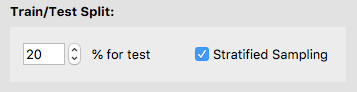
We will be using the holdout validation method in the software. This reserves a single fixed portion of the data for evaluation.
We will use the software’s default of 20% of the training set for the validation set.
Select Next to proceed to Step 2.

Step 2: Train classifiers
Classification is a process where given some input we are try to predict an outcome by coming up with a rule that will guess this outcome. Tools that use classification to predict an outcome are classifiers.
Definitions
Classification - The task in supervised learning when the label is a category. The goal of classification is to predict which category each sample belongs to.
Classifier - A specific model or algorithm which performs classification.
Regression - The task in supervised learning when the label is numeric. Instead of predicting a category, here the value of the label variable is predicted.
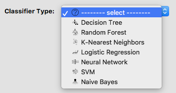
Software
The software has a dropdown menu of some of the most frequently used classifiers. Choose one of them to continue with for this lesson.
In this workshop, we will be further talking about [Decision Trees][episode-trees-overfitting], [Random Forests][episode-trees-overfitting], [Logistic Regression][episode-logit-ann], and [Artificial Neural Networks][episode-logit-ann].
Each classifier has its own hyperparameters specific to that classifier that can be tuned. Intuitively, think of the hyperparameters as the “knobs and dials” or settings of the classifier. You can adjust the hyperparameters and explore how they impact performance on the training and validation sets. If you train an SVM, you will have to increase the max_iter parameter to be at least 1000.

You may give your classifier a name and add a comment. If you do not specify a name, the software will use “classifier_[int]” as its default name. For example, if the classifier is the third one you trained, its default name is “classifier_3”.
Software
If you changed the hyperparameters but want to start over, click on Reset. The hyperparameters will be back to default. Otherwise, click on Train.
We will use accuracy to evaluate the classifiers. Accuracy measures the fraction of the predictions that are correct. In the T-cells dataset, this is the number of correctly predicted quiescent and activated cells compared to the total number of predictions made.
Software
In the software, look at the prediction metrics on the validation data.
Remember, you can switch between the training set and validation set at any time.
In the T-cells example, we want to predict whether a cell was quiescent or activated. The accuracy gives us the count of the cells that were correctly predicted.
This type of exploration of multiple algorithms reflects how a good model is often found in real-world situations. It often takes many classifiers to find the one that you are satisfied with.
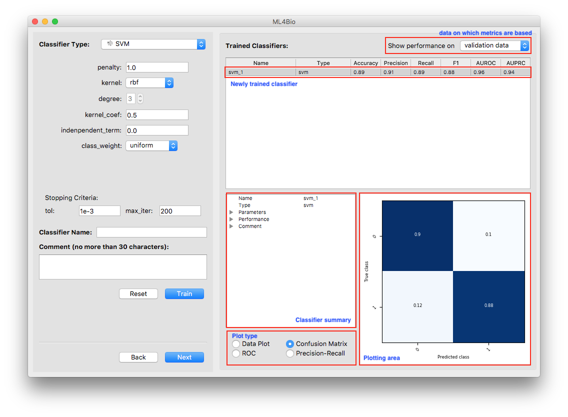
At the bottom right of the software window, there is a variety of information about the trained model.
Three types of plots that reflect the classifier’s performance are always available. The data plot is only available when the dataset contains exactly two continuous features. Note that the plots are all with respect to the type of data shown at the top-right corner of the software window.
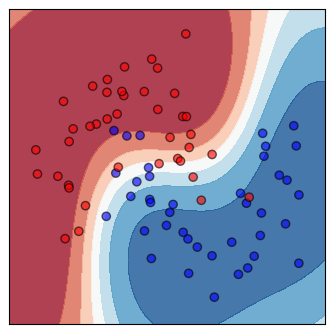
Shown on the top is a scatter plot of the training data and contours of the decision regions. This is a visualization of the decision boundary of the classifier. The darker the color, the more confident the classifier is.
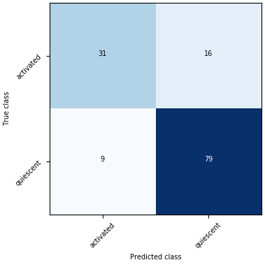
Shown on the bottom is the confusion matrix. The Confusion Matrix reflects the selected dataset (training or validation). The T-cells dataset has two labels so that the Confusion Matrix will be 2 x 2. The sum of all the predictions will be the total number of samples in the selected dataset (training or validation).
Software - Poll
Train a few different classifiers and explore the following questions:
How does the decision boundary change as the classifier and hyperparameters change?
What is the highest validation set accuracy you can achieve?
How does this compare to the training set accuracy?
Definitions
Decision boundary - A region where all the patterns within the decision boundary belong to the same class. It divides the space that is represented by all the data points. Identifying the decision boundary can be used to classify the data points. The decision boundary does not have to be linear.
Confusion matrix - A matrix used in classification to visualize the performance of a classifier. Each cell shows the number of time the predicted and actual classes of samples occurred in a certain combination.
Step 3 Test and Predict
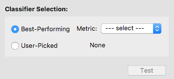
Our final step is model selection and evaluation. After we trained multiple classifiers and did holdout validation, the next step is to choose the best model. Hit Next to continue.
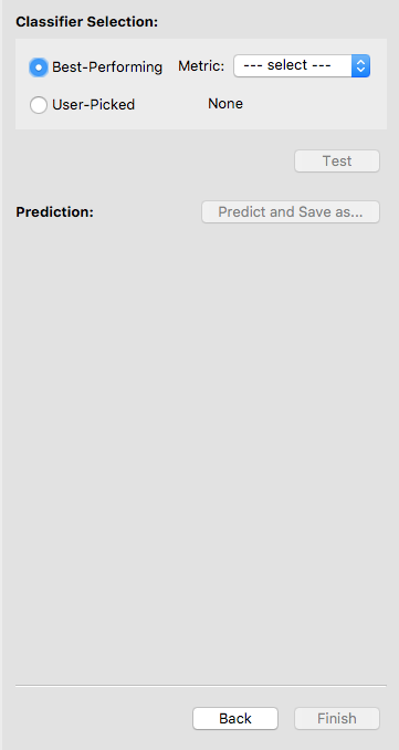
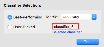
To select a classifier, you may let the software pick one for you by specifying a metric. In this case, the software will select the best classifier with respect to that metric. Otherwise, you may pick a classifier on your own. We let the software select the classifier with the highest accuracy.
After a classifier is selected, its name will show up. Double-check that it is the one you want to test. Now the Test button is enabled, and you may click on it to test the selected classifier. Note that once you hit Test, you are no longer allowed to go back and train more classifiers.
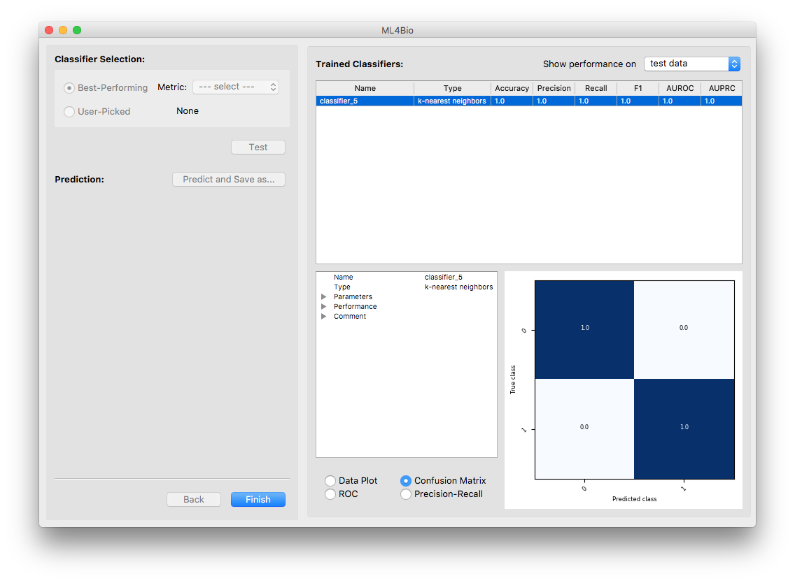
Now the only classifier in the list is the tested one. Note that the software is showing the classifier’s performance on the test data. You may examine the performance using either the summary or the plots.
Questions to consider
How did your final test set accuracy compare to your validation accuracy?
Image attributions
The T-cell images come from Wang et al. 2019 with data originally from Walsh et al. 2020.
Break
Let’s take a short break.
- The ml4bio software supports interactively exploring different classifiers and hyperparameters on a dataset
- The machine learning workflow is split into data preprocessing and selection, training and model selection, and evaluation stages
- Splitting a dataset into training, validation, and testing sets is key to being able to properly evaluate a machine learning method
Content from Evaluating a Model
Last updated on 2026-02-12 | Edit this page
Overview
Questions
- How do you evaluate the performance of a machine learning model?
Objectives
- Create questions to ask about a machine learning task to aid model selection
- Choose the appropriate evaluation metric for a particular machine learning problem
- Derive the definitions of popular evaluation metrics
Evaluation Metrics
Arguably the most important part of choosing a model is evaluating it to see how well it performs. So far we’ve been looking at metrics such as accuracy, but let’s take a look at how we think about metrics in machine learning.
In the binary classification setting (where there are only two classes we’re trying to predict, such as activated or quiescent T-cells) we can group all possible predictions our classifier makes into four categories. This is organized into a table called the confusion matrix:

Here, all possible types of predictions are split by 1) What the actual, true class is and 2) what the predicted class is, that is, what our classifier thinks the truth is. This results in the 4 entries of the confusion matrix, two of which means our classifier got something right:
Definitions
True Positives (TP): These instances are actually true (activated) and have been correctly predicted to be true.
True Negatives (TN): These instances are actually false (quiescent) and have been correctly predicted to be false.
And two of which means our classifier got something wrong:
Definitions
False Positives (FP) - These are instances which are actually false but our classifier predicted to be true. False positives are sometimes called type I errors or \(\alpha\) errors.
False Negatives (FN) - These are instances which are actually true but our classifier predicted to be false. False negatives are sometimes called type II errors or \(\beta\) errors.
Almost all evaluation metrics used in machine learning can be derived from the entries in the truth table, typically as a ratio of two sets of entries. For instance, accuracy is defined as the percent of instances the classifier got right.
So to calculate accuracy we take the number of things we got right, which is the number of true positives and the number of true negatives:

And divide it by the number total entries in the table, which is all four entries:

Therefore, accuracy is defined as \(\frac{TP + TN}{TP+FP+TN+FN}\).
We can see accuracy as estimating the answer to the question How likely is our classifier to get a single instance right? However, for many models this might not be the right question.
An example of a different question we might want to ask about a model would be If our classifier predicts something to be true, how likely is it to be right?
To answer this question we would look at everything we predicted to be true, which is the true positive and false positives:

We would then calculate the percent of these predictions that were correct, which are the true positives. Thus, to answer this question we would use the metric \(\frac{TP}{TP + FP}\).
This metric is called precision in machine learning (and may be different from the definition of precision you use in a laboratory setting).
Scenario 1 - Poll
You are designing a long-term study on the mutational rates of various breast cancer subtypes over several years using cell lines. Due to cost constraints you can only choose a few cell lines to monitor. However, there has been some recent research calling into question whether or not certain cell lines you were considering using are actually the cancer subtype they are believed to be. You cannot afford to include cell lines of the wrong subtype in your study. To aid in this task you decide to create a machine learning system to help verify that the cells lines you want to use are, in fact, the cancer subtypes you want to study. The model uses gene expression data to predict cancer subtype.
- Which entries in the confusion matrix are most important in this machine learning task? Is one type of correct or one type of incorrect prediction more important than the other for your machine learning system?
- Which metric would you use to evaluate this task?
Scenario 2 - Poll
You are designing a machine learning system for discovering existing drugs which may be effective in treating Malaria, focusing on the parasite Plasmodium falciparum. Your system takes in information on an FDA approved drug’s chemical structure, and predicts whether or not a drug may interact with P. falciparum. The machine learning system will be used as an initial screening step; drugs classified as interacting by your system will be flagged and tested in the lab. It is okay if some drugs sent to be tested in the lab end up having no effect. If your study leads to the approval of even a single new drug for treating P. falciparum you will consider the system a success. The vast majority of drugs will not be useful in treating P. falciparum.
- Which entries in the confusion matrix are most important in this machine learning task? Is one type of correct or one type of incorrect prediction more important than the other for your machine learning system?
- Imagine a classifier that predicted that all drugs are non-interacting. If you evaluated this classifier using the entire catalog of FDA approved drugs, what would the accuracy look like?
- What metric or couple of metrics would you use to evaluate your machine learning system?
Load the
simulated_drug_discovery/simulated-drug-discovery.csv
dataset from the data folder into the ML4Bio software. Try
training a logistic regression classifier on the dataset. Which metrics
seem to accurately reflect the performance of the classifier?
Common Metrics:
| Name | Formula |
|---|---|
| Accuracy | \(\frac{TP + TN}{TP+FP+TN+FN}\) |
| Precision (Positive Predictive Value) | \(\frac{TP}{TP + FP}\) |
| Recall (Sensitivity, True Positive Rate) | \(\frac{TP}{TP + FN}\) |
| True Negative Rate (Specificity) | \(\frac{TN}{TN + FP}\) |
| False Positive Rate | \(\frac{FP}{FP + TN}\) |
| F1 Score | \(\frac{2TP}{TP + TN + FP + FN}\) |
Error Curves
When evaluating machine learning models, multiple metrics are often combined into curves to be able to summarize performance into a single final metric. These curves are plotted at different confidence cut-offs, selecting different confidence thresholds for what is predicted to be in the positive class. The two most popular curves are the ROC curve and the PR curve.
{% include pr_curve_slideshow.html %}
Definitions
Receiver Operating Characteristic (ROC) Curve - A curve which plots the recall (true positive rate) against the false positive rate at different confidence cut-offs. The area under the curve (often called the AUROC) can then be used as a single metric to evaluate a classifier.
Precision Recall (PR) Curve - A curve which plots the precision against the recall at different confidence cut-offs. The area under the curve (often called AUPR) can then be used as a single metric to evaluate a classifier.
- The choice of evaluation metric depends on the relative proportions of different classes in the data, and what we want the model to succeed at.
- Comparing performance on the validation set with the right metric is an effective way to select a classifier and hyperparameter settings.
Content from Decision Trees, Random Forests, and Overfitting
Last updated on 2026-02-12 | Edit this page
Overview
Questions
- How do decision trees and random forests make decisions?
Objectives
- Describe the decision boundary of a decision tree and random forest
- Understand advantages and disadvantages of decision trees and random forests
- Identify evidence of overfitting
What is the decision tree classifier?
Decision trees make predictions by asking a sequence of questions for each example and make a prediction based on the responses. This makes decision trees intuitive. One of the benefits is that we can clearly see the path of questions and answers we took to get to the final prediction. For example, a doctor might use a decision tree to decide which medicine to prescribe based on a patient’s responses about their symptoms. Or in the case of T-cells, a decision tree can predict whether a T-cell is active or quiescent.
Example
To better understand the algorithm, consider the classification task of predicting whether a house has a low or high price. If the house price is higher than $200k, we will predict high, otherwise we will predict low. We are going to begin with an initial house price range, and for our neighborhood of interest the prices range from $100k - $250k. The first question we could ask is the number of bedrooms in the house. The answer is 3 bedrooms, and so our new range will be $180k-$250k. Then, we will ask about the number of bathrooms, and the answer is 3 bathrooms. The new range is $220-$250. Finally, we will ask the house’s neighborhood. The answer is Neighborhood A. That gives us the price of $230k. Our final class label is high.


How does the classifier make predictions?
Each split of a decision tree classifies instances based on a test of a single feature. This test can be True or False. The splitting goes from the root at the top of the tree to a leaf node at the bottom.
Definitions
Root node - the topmost node where the decision flow starts.
Leaf node - a bottom node that doesn’t split any further. It represents the class label.
An instance is classified starting from the root and testing the feature specified by the node, then going down the split based on the outcome of the test and testing a different feature specified by another node. Each leaf node in the tree is a class label.
Definition
Node - a test performed on a feature. It splits into two branches.
About the classifier
A decision tree is a supervised learning classifier. It splits the initial population depending on a certain rule. The goal of the classifier is to predict the class label on a new set of data based on the rule that the classifier learned from the features of the training examples. An important property of the decision tree is the depth of tree.
Definition
Depth of tree - the number of times we make a split to reach a decision.
Some pros of using decision trees:
- often simpler to visualize and interpret than other models
- the classification can be visually followed and performed manually
- makes few assumptions about the data
- can ignore useless features
Some cons of using decision trees:
- prone to overfitting
- requires a way to turn numeric data into a single decision rule
Definition
Overfitting - an overfitting model fits the training data too well, but it fails to do this on the new data.
Select data
Software
Load simulated_t_cell/simulated_t_cells_7.csv data set
into the software.
Turn off “stratified sampling” under validation methodology (right above next) before continuing.
Conceptual Questions
What are we trying to predict?
We will continue working on the T-cells example. The goal is the same, predicting whether a cell is active or quiescent. We also have the same two features: cell size and intensity.
Train classifiers
In the original T-cells example, we left the hyperparameters settings as the defaults. Now we will look further into some of the hyperparameters. In this workshop, not all of the hyperparameters from the software will be covered. For the hyperparameters that we don’t discuss, use the default settings.
- Max_depth can be an integer or None. It is the maximum depth of the tree. If the max depth is set to None, the tree nodes are fully expanded or until they have less than min_samples_split samples.
- Min_samples_split and min_samples_leaf represent the minimum number of samples required to split a node or to be at a leaf node.
- Class_weight is important hyperparameter in biology research. If we had a training set and we are using binary classification, we don’t want to only predict the most abundant class. For example, in the T-cells example, if 2 samples are active and 98 samples are quiescent, we don’t want to train a model that predicts all of the cells to be quiescent. Class_weight parameter would allow putting weight on 2 cells labeled as active so that predicting them incorrectly would be penalized more. In biology, it is common to have this type of imbalanced training set with more negative than positive instances, so training and evaluating appropriately is essential! The uniform mode gives all classes the weight one. The balanced mode adjusts the weights.
Definition
Imbalanced training set - a data set that contains a large proportion of a certain class or classes.
Software
Train a decision tree with the default hyperparameter settings, then look at the Data Plot.
Conceptual Questions
What is the decision boundary?
If we look at the Data Plot, the decision boundaries are rectangular.
Question
What do the individual line segments which make up the decision boundary represent?
They each represent a node in the decision tree. The line segment shows the split at that node.
Conceptual Question
What hyperparameter might be important for this example? (hint: what is not ideal about this dataset?)
Software
One thing we can see from the data plot is that this dataset is imbalanced, with more quiescent cells than active cells. Let’s change the class_weight hyperparameter to balanced.
Activity
Did this make any difference?
How does the data plot look for the uniform class_weight and how does it look for the balanced class weight?
Random Forests
Random forests deals with the problem of overfitting by creating multiple trees, with each tree trained slightly differently so it overfits differently. Random forests is a classifier that combines a large number of decision trees. The decisions of each tree are then combined to make the final classification. This “team of specialists” approach random forests take often outperforms the “single generalist” approach of decision trees. Multiple overfitting classifiers are put together to reduce the overfitting.
Motivation from the bias variance trade-off

If we examine the different decision boundaries, note that the one of the left has high bias while the one on the right has high variance.
{% include biasvariance_slideshow.html %}
Definitions
Bias - The assumptions made by a model about what the decision boundary will look like. Models with high bias are less sensitive to changes in the training data.
Variance - The amount the training data affects what a model’s decision boundary looks like. Models with high variance have low bias.
Note that these concepts have more exact mathematical definitions which are beyond the scope of this workshop.
Random forests are based on mitigating the negative effects of this trade-off by creating multiple high variance models that work together.
Why is it called “random” forests?
If when training each tree in the forest, we give every tree the same data, we would get the same predictions that are prone to overfitting. In order to train the decision trees differently we need to provide slightly different data to each tree. To do this, we choose a random subset of the data to give to each tree. When training at each node in the tree we also randomize which features can be used to split the data. This method of creating random subsamples of data to make an ensemble of classifiers which are then combined is called bagging. The final prediction is based on a vote or the average taken across all the decision trees in the forest.

Definitions
Ensemble method - A general method where multiple models are combined to form a single model.
Bagging - An ensemble method where many training sets are generated from a single training set using random sampling with replacement. Models are then trained on each sampled training set and combined for a final prediction. It is short for bootstrap aggregating.
Overfitting Example
Software - Poll
Load t_cell/cellprofiler_feature.csv data set into the
software.
Try training both a decision tree and a random forest on the data.
What do you notice after you trained the model?
How did the classifier perform on the training data compared to the validation data?
Try training a decision tree with the max_depth hyperparameter set to 2.
Did you notice any difference?
A good model will learn a pattern from the data and then it will be able to generalize the pattern on the new data.
It is easy to go too deep in the tree, and to fit the parameters that are specific for that training set, rather than to generalize to the whole dataset. This is overfitting. In other words, the more complex the model, the higher the chance that it will overfit. The overfitted model has too many features. However, the solution is not necessarily to start removing these features, because this might lead to underfitting.
The model that overfits has high variance.
Software
To check if the classifier overfit, first look at the training data.
Switch between training data and validation data in the upper right corner.
By looking at the evaluation metrics and the confusion matrix we can see that when the training data evaluation metrics were perfect, but they were not as great on the validation data. The classifier probably overfit.
Software
Let’s go to the Step 3 in the software.
Questions
Based on accuracy, which classifier was best-performing?
Did the classifier overfit?
Classifier selection scenarios - Poll
In the following scenarios, which classifier would you choose?
You want to create a model to classify a protein’s subcellular localization (nucleus, mitochondria, plasma membrane, etc.). You have a labeled set of 15,000 human proteins with 237 features for each protein. These features were computationally derived from simulations using protein structure predicting software, and do not have any predefined meaning. Thus, you do not expect the features to be meaningful for human interpretation.
You want to create a model to predict whether or not a species’ conservation status (least concern, endangered, extinct, etc.) will be affected by climate change. You have a labeled dataset of 40 species, with 18 features for each species which have been curated by ecologists. These features include information such as the species’ average size, diet, taxonomic class, migratory pattern, and habitat. You are interested to see which features are most important for predicting a species’ fate.
Application in biology
PgpRules: a decision tree based prediction server for P-glycoprotein substrates and inhibitors
- Decision trees require less effort to visualize interpret than other models
- Decision trees are prone to overfitting
- Random forests solve many of the problems of decision trees but are more difficult to interpret
Content from Logistic Regression, Artificial Neural Networks, and Linear Separability
Last updated on 2026-02-12 | Edit this page
Overview
Questions
- What is linear separability?
Objectives
- Understand advantages and disadvantages of logistic regression and artificial neural networks
- Distinguish linear and nonlinear classifiers
- Select a linear or nonlinear classifier for a dataset
Logistic Regression
Logistic regression is a classifier that models the probability of a certain label. In the T-cells example, we were classifying whether cells were in the two categories of active or quiescent. Using the logistic regression to predict the whether a cell is active is a binary logistic regression. Everything that applies to the binary classification could be applied to multi-class problems (for example, if there was a third cell state). We will be focusing on the binary classification problem.
Linear regression vs. logistic regression
We can write the equation for a line as \(y=mx+b\), where \(x\) is the x-coordinate, \(y\) is the y-coordinate, \(m\) is the slope, and \(b\) is the intercept. We can rename \(m\) and \(b\) to instead refer to them as feature weights, \(y=w_1x+w_0\). Now \(w_0\) is the intercept of the line and \(w_1\) is the slope of the line. In statistics, for the simple linear regression we write intercept term first \(y=w_0+w_1x\).
Definition
Feature weights - determine the importance of a feature in a model.
The intercept term is a constant and is defined as the mean of the outcome when the input \(x\) is 0. This interpretation gets more involved with multiple inputs, but that is out of the scope of the workshop. The slope is a feature weight. In the T-cells example, the feature weight is the coefficient for the feature \(x\) and it represents the average increase in the confidence the cell is active with a one unit increase in \(x\).
When we have multiple features, the linear regression would be \(y = w_0 + w_1x_1 + w_2x_2 +...+ w_nx_n\).

What is logistic regression?
Logistic regression returns the probability that a combination of features with weights belongs to a certain class.
In the visual above that compares linear regression to logistic regression, we can see the “S” shaped function is defined by \(p = \frac{1}{1+e^{-(w_0+w_1x_1)}}\). The “S” shaped function is the inverse of the logistic function of odds. It guarantees that the outcome will be between 0 and 1. This allows us to treat the outcome as a probability, which also must be between 0 and 1.
Definition
Odds - probability that an event happens divided by probability that an event doesn’t happen.
\(odds = \frac{P(event)}{1-P(event)}\)
Now, let’s think about the T-cells example. If we focus only on one feature, for example cell size, we can use logistic regression to predict the probability that the cell would be active.
The logistic function of odds is a sum of the weighted features. Each feature is simply multiplied by a weight and then added together inside the logistic function. So logistic regression treats each feature independently. This means that, unlike decision trees, logistic regression is unable to find interactions between features. An example of a feature interaction is if the copy number increase of a certain gene may only affect cell state if another gene is also mutated. This feature independence affects what type of rules logistic regression can learn.
Questions to consider
What could be another example of two features that interact with each other?
An important characteristic of features in logistic regression is how they affect the probability. If the feature weight is positive then the probability of the outcome increases, for example the probability that a T-cell is active increases. If the feature weight is negative then the probability of the outcome decreases, or in our example, the probability that a T-cell is active decreases.
Definition
Linear separability - drawing a line in the plane that separates all the points of one kind on one side of the line, and all the points of the other kind on the other side of the line.
Recall, \(y=mx+b\) graphed on the coordinate plane. It is a straight line. \(y = w_0 + w_1x_1\) is a straight line. The separating function has the equation \(w_0+w_1x_1= 0\). If \(w_0+w_1x_1>0\) the T-cell is classified as active, and if \(w_0+w_1x_1<0\) the T-cell is classified as quiescent.
Questions to consider
When do you think something is linearly separable?
You can use the TensorFlow Playground website to explore how changing feature weights changes the line in the plane that separates blue and orange points. This example has two features \(x_1\) and \(x_2\). You can click the the blue lines to modify the weights \(w_1\) and \(w_2\). Press the play button to automatically train the weights to minimize the number of points that are predicted as the wrong color.
Step 1 Train a Logistic Regression Classifier
Software
Load the toy_data/toy_data_3.csv data set into the
software.
This dataset is engineered specifically for the logistic regression classifier.
Linear separability
In this workshop, not all of the hyperparameters in the ml4bio software will be discussed. For those hyperparameters that we don’t cover, we will use the default settings.
Software
Let’s train a logistic regression classifier.
For now use the default hyperparameters.
Questions to consider - Poll
Look at the Data Plot. What do you notice?
Is the data linearly separable?
Logistic regression can also be visualized as a network of features feeding into a single logistic function.

At the logistic function, the connected features are combined and fed into the logistic function to get the classifier’s prediction. In this visualization, we can see that the features never interact with each other until they reach the logistic function, which results in feature independence.
Artificial Neural Networks
An artificial neural network can be viewed as an extension of the logistic regression model, where additional layers of feature interactions are added. These additional layers allow for more complex, non-linear decision boundaries to be learned.

Artificial neural networks have inputs and outputs, just like logistic regression, but have one or more additional layers called hidden layers comprised of hidden units. Hidden layers can contain any number of hidden units. In the neural network diagram, each unit in the input, output, and hidden layers resemble neurons in a human brain, hence the name neural network. The above figure shows a fully connected hidden layer, where every feature interacts with every other feature to form a new value. The new value is created by passing the sum of the weighted feature values into the activation function of the hidden layer. These new values are then fed to the logistic function as opposed to the raw features.
Definitions
Hidden unit - a function in a neural network that takes in values, applies some function to them, and outputs new values to be used in subsequent layer of the neural network.
Hidden layer - a layer of hidden units in a neural network, such as the logistic function.
Activation function - the function used to combine values in a specific layer of a neural network.
You can again use TensorFlow Playground to examine the difference between logistic regression, which has a single logistic function, and a neural network with multiple hidden layers. This example initially attemps to use logistic regression to separate the orange and blue points. Try adding more hidden layers and more neurons in each layer using the play button to train the weights.
This final example has a complicated orange/blue pattern. Press the play button to watch how the neural network can iteratively make small weight updates that reduce the number of mislabeled points.
Step 2 Compare Linear and Nonlinear classifiers
Software
Load the toy_data/toy_data_8.csv data set into the
software.
This data set is engineered specifically to demonstrate the difference between linear and nonlinear classifiers.
Train a logistic regression classifier using the default hyperparameters.
Questions to consider
What are the evaluation metrics telling us?
Look at the Data Plot. What do you notice?
Is the data linearly separable?
Software
Now train a neural network on the same data.
Questions to consider
What shape is the decision boundary?
How did the performance of the model change on the validation data?
This example demonstrates that logistic regression performs great with data that is linearly separable. However, with the nonlinear data, more complex models such as artificial neural networks need to be used.
Artificial neural networks in practice
Artificial neural networks with a single hidden layer tend to perform well on simpler data, such as the toy datasets in this workshop.
However artificial neural networks used on more complex data, such as raw image data or protein structure data, typically have much more complex architectures.
For example, below is the architecture of a neural network used to evaluate the skill of robotic surgery arms based on motion captured over time.
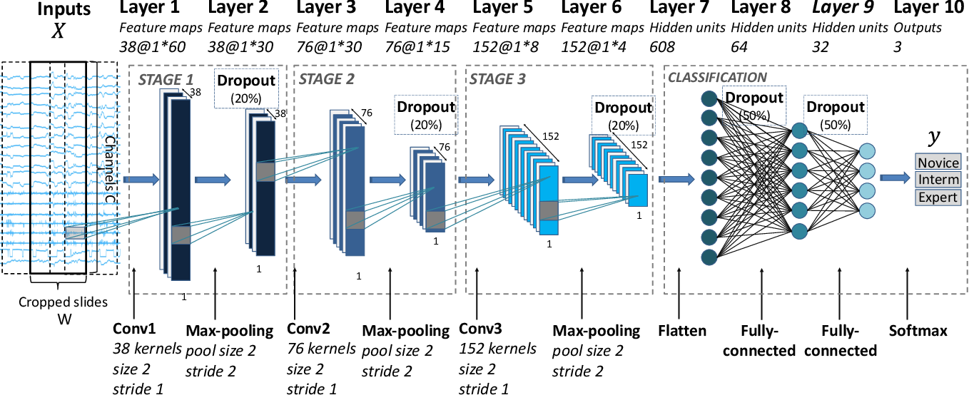
This neural network still consists of hidden layers combined with functions, but contains many specialized layers which perform specific operations on the input features.
Classifier selection scenarios - Poll
In the following scenarios, which classifier would you choose?
You are interested in learning about how different factors contribute to water preservation adaptations in plants. You plan to create a model for each of 4 moisture preservation adaptations, where in each model the presence of the moisture preservation adaptation is the class being predicted. You use a dataset of 200 plant species to train each model. You have 15 features for each species, consisting of environmental information such as latitude, average temperature, average rainfall, average sun intensity, etc.
You have been tasked with creating a model to predict whether a mole sample is benign or malignant based on gene expression data. Your dataset is a set of 380 skin samples, each of which has expression data for 50 genes believed to be involved in melanoma. It is likely that a combination of genes is required for a mole to be cancerous.
Step 3 Test Regularization Strategies
Regularization
Regularization is used to make sure that our model pays attention only to the important features to avoid overfitting. Previously, we talked about the positive and negative effect a feature and its weight can have on the outcome probability. As with decision trees and random forests, logistic regression can overfit. If we have a complex model with many features, our model might have high variance. Regularization can help us decide how many features are too many or too few. Regularization does not make models fit better on the training data, but it helps with generalizing the pattern to new data.
Definition
Regularization - approaches to make machine learning models less complex in order to reduce overfitting.
Penalty - a regularization strategy that reduces the importance of certain features by adding a cost to the feature weights, which makes the feature weights smaller.
Regularization hyperparameters in the ml4bio software
The most important hyperparameters in the ml4bio software are:
- The regularization penalty can be L1 or L2. Although it is possible to train a logistic regression classifier without regularization, regularization is always used in the ml4bio software. This follows best practices in real applications.
- C is the inverse of the regularization strength. Smaller values of C mean stronger regularization (higher penalties, therefore lower feature weights).
Software
Load the simulated_t_cell/simulated_t_cells_1.csv data
set into the software.
This data set is engineered specifically to demonstrate the effects of regularization.
L1 regularization
L1 regularization is also known as Lasso regularization.
Recall that \(x_1, x_2, ..., x_n\) are the features, and \(w_0, w_1, ..., w_n\) are the feature weights. Without regularization, the classifier might fit the training data perfectly, giving certain values to each weight that would lead to overfitting. This model could be very complex and it would generalize poorly on the future data.
L1 regularization prevents overfitting by adding a penalty term and mathematically shrinking (decreasing) some weights. L1 could shrink the weights of less important features all the way to 0, effectively deleting those weights. The corresponding features are then not used at all to make predictions on new data.
L2 Penalty
L2 regularization is also known as ridge regularization. L2 regularization makes the weights of less important features to be small values. Unlike L1 regularization, L2 regularization does not necessarily shrink the weights to 0. The higher the value of C, the smaller the feature weights will be.
Recall: C is the inverse of regularization strength. Smaller values of C will shrink more weights and use fewer features to make the prediction.
Software
First, set penalty to ‘L1’. Experiment with C = 0.001, 0.07, 0.1, 0.25, 1.
Next, set penalty to ‘L2’. Experiment with the same values of C.
Questions
What do you observe in the Data Plot? For each value of C, which of the two features seem to influence the decision boundary?
What is the difference between L1 and L2 regularization? (Hint: consider C = 0.07)
How does the decision boundary change as C increases?
L1 can regularize such that one feature’s weight goes to 0. We can see the classifier ignores that feature in its decision boundary.
Break
Let’s take a short break.
- Logistic regression is a linear classifier.
- The output of logistic regression is probability of a certain class.
- Artificial neural networks can be viewed as an extension of logistic regression
- Artificial neural networks can have nonlinear decision boundaries
Content from Understanding Machine Learning Literature
Last updated on 2026-02-12 | Edit this page
Overview
Questions
- How are machine learning workflows presented in research papers?
Objectives
- Assess a typical machine learning methodology presented in an academic paper
This lesson will focus on understanding and evaluating machine learning workflows as they are presented in the literature. For this lesson, you will choose one of the below papers to read. Please read this paper for day 2 of the workshop, so you are familiar with the paper’s layout. Alternatively, if you brought a paper to day 1 you think is a good candidate, we can add it to the list of papers people can choose from. We will ask you to switch papers if you end up being the only person in the workshop who chooses that paper.
We will be exploring filling out this chart for the paper you select. This chart is a tool to help you think about how machine learning is used in a paper and come to a conclusion about if you think the claims made in the paper using machine learning are valid.
Choosing a paper to read
The paper you choose will use supervised learning in some form. While the paper should contain a classification or regression task, this task does not have to be the main goal of the paper. If the paper you choose has multiple machine learning models or tasks, choose one of them to focus on.
Terms to look out for when searching for a paper are terms related to the machine learning workflow such as training, testing, holdout, features, classifier, or regression. You can also looks for the name of a specific classifier, such as random forest or neural network. Papers which use deep learning methods are also usable for this activity.
It’s okay if the paper is not an exact fit, especially if it is a technique used in your field which you want to understand.
Example/Backup Papers
Here is a list of papers which you can choose for this activity.
- Classification of human genomic regions based on experimentally determined binding sites of more than 100 transcription-related factors
- DeepCpG: accurate prediction of single-cell DNA methylation states using deep learning
- Gradient modeling of conifer species using random forests
- A Logistic Regression Model Based on the National Mammography Database Format to Aid Breast Cancer Diagnosis
- Potential neutralizing antibodies discovered for novel corona virus using machine learning
- seqQscorer: automated quality control of next-generation sequencing data using machine learning
- Identifying mouse developmental essential genes using machine learning
- A deep learning approach to antibiotic discovery
Example Chart
While it might be helpful to look at this chart while filling out the paper, you do not need to fill this chart out before day 2 of the workshop. You will fill out this chart for the paper you chose during day 2 of the workshop.
Here is an example partially filled-out chart from Predictive Models for Breast Cancer Susceptibility from Multiple Single Nucleotide Polymorphisms. Note that this paper uses 3 different classifiers, but we are just going to focus on the decision tree:

Example Chart Activity
Look in the paper for where the filled in parts of the chart came from.
Based on the paper and the filled out parts of the chart, try to fill in the Your Conclusions section.
Charting Your Paper
Now, on your own, see if you can fill in a blank chart using the paper you brought today with your group.
- Research workflows for machine learning are often not straightforward
- Published papers often omit details which can make it difficult to evaluate machine learning workflows
- Machine learning is used in a large variety of ways in biology
Content from Conclusion and next steps
Last updated on 2026-02-12 | Edit this page
Overview
Questions
- Where can you learn more about machine learning?
Objectives
- Assess how well you understand a machine learning workflow
- Provide feedback on the workshop
- Discuss additional machine learning resources
Model Selection
Choosing the proper machine learning model for a given task requires knowledge of both machine learning models and the domain of the task. Finding the best model for a new task in machine learning is often a research question in itself. Finding a model that performs reasonably well, however, can often be accomplished by carefully considering the task domain and a little trial and error with the validation set.
Some of the questions to consider when choosing a model are:
- How much data is there to train with?
- Does the data contain roughly the same number of instances from each class?
- How many features does the dataset have? Are all of the features relevant, or might some of them not be related to the data’s class?
- What types are the features (numeric, categorical, image, text)?
- What might the decision boundary look like? Is the data likely linearly separable?
- How noisy is the data?
Reviewing a published workflow
We will review a machine learning workflow from a publication to see how well you can identify the major elements that were presented during this workshop.
Post-workshop survey
We greatly appreciate your feedback to help improve this workshop. Please take 10 minutes to complete the post-workshop survey using the link you were provided.
Additional resources
The [References][lesson-reference] page links to additional resources on machine learning concepts and introductory tools. It includes a Jupyter notebook that shows Python code to execute the type of machine learning workflow you ran with the ml4bio software. The [Glossary][lesson-glossary] contains definitions of the machine learning terms used in this workshop. You can also use the additional real and simulated datasets that you downloaded to continue exploring how compatible different types of classifiers are with different data patterns.
- You are now prepared to consider how machine learning may benefit your research.
- There are many excellent introductory and intermediate resources to help you continue to learn about machine learning.