Homologous BGC Clusterization
Last updated on 2026-02-20 | Edit this page
Overview
Questions
- How can I identify Gene Cluster Families?
- How can I predict the production of similar metabolites
- How can I clusterize BGCs into groups that produce similar metabolites?
- How can I compare the metabolic capability of different bacterial lineages?
Objectives
- Understand the purpose of using
BiG-SLiCEandBiG-FAM - Learn the inputs required to run
BiG-SLiCEandBiG-FAM - Run an example with our Streptococcus data on both softwares
- Understand the obtained results
BiG-SLiCE and BiG-FAM a set of tools to compare the microbial metabolic diversity
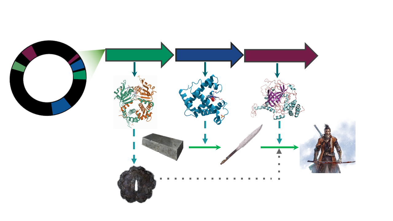
Around the curriculum, we have been learning about the metabolic capability of bacteria lineages encoded in BGCs. Before we start this lesson, let’s remember that the products of these clusters are biomolecules that are (mostly) not essential for life. They take the role of “tools” that offer some ecological and physiological advantage to the bacterial lineage producing it.
The presence/absence of a set of BGCs in a genome, can be associated to the ecological niches and (micro)environments which the lineage faces.
The counterpart of this can be taken as how biosynthetically diverse a bacterial lineage can be due to its environment.
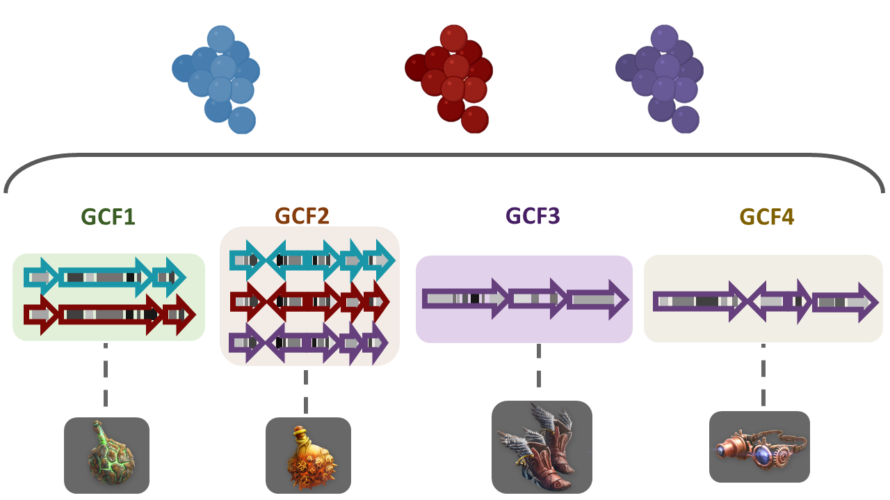
To answer some of this questions, we need a way to compare the metabolic capabilities of a set of diverse bacterial lineages. One way to do this is to compare the state (identity) of homologous BGCs. The homologous clusters that share a similar domain architecture and in consequence will produce a similar metabolite, are grouped into a bigger group that we call Gene Cluster Families (GCFs).
There are some programs capable of clustering BGCs in GCFs,
e.g.ClusterFinder and
DeepBGC.
BiG-SLICE is a software that has been designed
to do this work in less time, even when dealing with large datasets (1.2
million BGCs). This characteristic makes it a good tool to compare the
metabolic diversity of several bacterial lineages.
The input for BiG-SLiCE
Firstly, activate the conda environment, where BiG-SLiCE
has been installed as well as all the softwares required for its
usage:
You will have now a (GenomeMining) label at the
beginning of the prompt line.
If we seek for help using the --help flag of
bigslice, we can get a first glance at the input that we
need:
OUTPUT
usage: bigslice [-i <folder_path>] [--resume] [--complete] [--threshold T]
            	[--threshold_pct <N>] [--query <folder_path>]
            	[--query_name <name>] [--run_id <id>] [--n_ranks N_RANKS]
            	[-t <N>] [--hmmscan_chunk_size <N>] [--subpfam_chunk_size <N>]
            	[--extraction_chunk_size EXTRACTION_CHUNK_SIZE] [--scratch]
            	[-h] [--program_db_folder PROGRAM_DB_FOLDER] [--version]
            	<output_folder_path>

                        	_________
 ___	_____|\____|\____|\ \____	\
|   \  |   	} 	} 	}  ___)_ _/__
| >  | _--/--|/----|/----|/__/  __||  __|
|   < | ||  __/ (  (| | \___/  /__/|  _|
| >  || || |_ | _)  ) |_ | |\  \__ | |__
|____/|_| \___/|___/|___||_| \____||____| [ Version 1.1.0 ]

Biosynthetic Gene clusters - Super Linear Clustering Engine
(https://github.com/medema-group/bigslice)

positional arguments:
BiG-SLiCE is asking for a folder as the input. It is
important to highlight that the bones of this folder are the BGCs from a
group of genomes that has been obtained by antiSMASH. In
its GitHub page,
we can search for an input folder template.
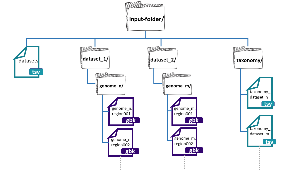
The folder needs three main components:
- datasets.tsv: This is a file that needs to have this exact name. This must be a tabular separated file where the information of each dataset (BGCs from a group of genomes) must be specified.

dataset_n: Each dataset will be composed by the BGCs of different genomes. We can give
BiG-SLiCEn groups of BGCs. The separation of the BGCs in different datasets is due to the different characteristics that the bacterial lineages can have. For example, if we have a set of bacterial populations that came from maize roots and other obtained from tomato roots, we can put them into dataset_1 and dataset_2 respectively.-
**taxonomy_n.tsv:**This is also a tabular separated file that will carry the taxonomic information of each of the genomes where the input BGCs were found and the path to reach these BGCs inside the input-folder:
- Genome folder name (ends with ‘/’)
- Kingdom / Domain name
- Class name
- Order name
- Family name
- Genus name
- Species name
- Organism / Strain name
Here, we have an example of the structure of the
input-folder:
Creating the input-folder
We will create a bigslice folder inside the
results directory.
Now that we know what input BiG-SLiCE requires, we will
do our input-folder step by step. First, let’s remember how many genomes
we have:
OUTPUT
agalactiae_18RS21/  agalactiae_A909/	agalactiae_COH1/
agalactiae_515/ 	agalactiae_CJB111/  agalactiae_H36B/
athermophilus_LMD-9/  athermophilus_LMG_18311/
We have six Streptococcus genomes from the original paper,
and two
public genomes. We will allocate their respective BGC .gbks
in two datasets, one for the genomes from Tettelin et
al. paper, and the other for the public ones.
BASH
$ mkdir input-folder
$ mkdir input-folder/dataset_1
$ mkdir input-folder/dataset_2
$ mkdir input-folder/taxonomy
$ tree
OUTPUT
.
└── input-folder
	├── dataset_1
	├── dataset_2
	└── taxonomy

4 directories, 0 files
Now we will create the folders for the BGCs of the dataset_1 genomes. We will take advantage of the strain name of our Streptococcus agalactiae lineages to create their folders:
BASH
$ for i in 18RS21 COH1 515 H36B A909 CJB111;
  do mkdir input-folder/dataset_1/Streptococcus_agalactiae_$i;
  done
$ tree -F
OUTPUT
.
└── input-folder/
	├── dataset_1/
	│   ├── Streptococcus_agalactiae_18RS21/
	│   ├── Streptococcus_agalactiae_515/
	│   ├── Streptococcus_agalactiae_A909/
	│   ├── Streptococcus_agalactiae_CJB111/
	│   ├── Streptococcus_agalactiae_COH1/
	│   └── Streptococcus_agalactiae_H36B/
	├── dataset_2/
	└── taxonomy/

10 directories, 0 files
We will do the same for the public genomes:
BASH
$ for i in LMD-9 LMG_18311;
  do mkdir input-folder/dataset_2/Streptococcus_thermophilus_$i;
  done
$ tree -F
BASH
.
└── input-folder/
	├── dataset_1/
	│   ├── Streptococcus_agalactiae_18RS21/
	│   ├── Streptococcus_agalactiae_515/
	│   ├── Streptococcus_agalactiae_A909/
	│   ├── Streptococcus_agalactiae_CJB111/
	│   ├── Streptococcus_agalactiae_COH1/
	│   └── Streptococcus_agalactiae_H36B/
	├── dataset_2/
	│   ├── Streptococcus_thermophilus_LMD-9/
	│   └── Streptococcus_thermophilus_LMG_18311/
	└── taxonomy/

12 directories, 0 files
Next, we will copy the BGCs .gbk files from the
dataset_1 genomes from each AntiSMASH output directory to
its respective folder .
BASH
$ ls input-folder/dataset_1/ | while read line;
  do cp ../antismash/output/$line/*region*.gbk input-folder/dataset_1/$line;
  done
$ tree -F
OUTPUT
.
└── input-folder/
	├── dataset_1/
	│   ├── Streptococcus_agalactiae_18RS21/
	│   │   ├── AAJO01000016.1.region001.gbk
	│   │   ├── AAJO01000043.1.region001.gbk
	│   │   └── AAJO01000226.1.region001.gbk
	│   ├── Streptococcus_agalactiae_515/
	│   │   ├── AAJP01000027.1.region001.gbk
	│   │   └── AAJP01000037.1.region001.gbk
	│   ├── Streptococcus_agalactiae_A909/
	│   │   ├── CP000114.1.region001.gbk
	│   │   └── CP000114.1.region002.gbk
	│   ├── Streptococcus_agalactiae_CJB111/
	│   │   ├── AAJQ01000010.1.region001.gbk
	│   │   └── AAJQ01000025.1.region001.gbk
	│   ├── Streptococcus_agalactiae_COH1/
	│   │   ├── AAJR01000002.1.region001.gbk
	│   │   └── AAJR01000044.1.region001.gbk
	│   └── Streptococcus_agalactiae_H36B/
	│   	├── AAJS01000020.1.region001.gbk
	│   	└── AAJS01000117.1.region001.gbk
	├── dataset_2/
	│   ├── Streptococcus_thermophilus_LMD-9/
	│   └── Streptococcus_thermophilus_LMG_18311/
	└── taxonomy/

12 directories, 13 files
Again, we will do the same for the BGCs .gbks of the
dataset_2:
BASH
$ ls input-folder/dataset_2/ | while read line;
  do cp ../antismash/output/$line/*region*.gbk input-folder/dataset_2/$line;
  done
$ tree -F
BASH
.
└── input-folder/
	├── dataset_1/
	│   ├── Streptococcus_agalactiae_18RS21/
	│   │   ├── AAJO01000016.1.region001.gbk
	│   │   ├── AAJO01000043.1.region001.gbk
	│   │   └── AAJO01000226.1.region001.gbk
	│   ├── Streptococcus_agalactiae_515/
	│   │   ├── AAJP01000027.1.region001.gbk
	│   │   └── AAJP01000037.1.region001.gbk
	│   ├── Streptococcus_agalactiae_A909/
	│   │   ├── CP000114.1.region001.gbk
	│   │   └── CP000114.1.region002.gbk
	│   ├── Streptococcus_agalactiae_CJB111/
	│   │   ├── AAJQ01000010.1.region001.gbk
	│   │   └── AAJQ01000025.1.region001.gbk
	│   ├── Streptococcus_agalactiae_COH1/
	│   │   ├── AAJR01000002.1.region001.gbk
	│   │   └── AAJR01000044.1.region001.gbk
	│   └── Streptococcus_agalactiae_H36B/
	│   	├── AAJS01000020.1.region001.gbk
	│   	└── AAJS01000117.1.region001.gbk
	├── dataset_2/
	│   ├── Streptococcus_thermophilus_LMD-9/
	│   │   ├── CP000419.1.region001.gbk
	│   │   ├── CP000419.1.region002.gbk
	│   │   ├── CP000419.1.region003.gbk
	│   │   ├── CP000419.1.region004.gbk
	│   │   └── CP000419.1.region005.gbk
	│   └── Streptococcus_thermophilus_LMG_18311/
	│   	├── NC_006448.1.region001.gbk
	│   	├── NC_006448.1.region002.gbk
	│   	├── NC_006448.1.region003.gbk
	│   	├── NC_006448.1.region004.gbk
	│   	├── NC_006448.1.region005.gbk
	│   	└── NC_006448.1.region006.gbk
	└── taxonomy/

12 directories, 24 filesExercise 1. Input-folder structure
As we have seen, the structure of the input folder for BiG-SLiCE is quite difficult to get. Imagine “Sekiro” wants to copy the directory structure to use it for future BiG-SLiCE inputs. Consider the following directory structure:
OUTPUT
  └── input_folder/
   	├── datasets.tsv
   	├── dataset_1/
   	|   ├── genome_1A/
   	|   |   ├── genome_1A.region001.gbk
   	|   |   └── genome_1A.region002.gbk
   	|   ├── genome_1B/
   	|   |   ├── genome_1B.region001.gbk
   	|   |   └── genome_1B.region002.gbk
   	├── dataset_2/
   	|   ├── genome_2A/
   	|   |   ├── genome_2A.region001.gbk
   	|   |   └── genome_2A.region002.gbk
   	|   ├── genome_2B/
   	|   |   ├── genome_2B.region001.gbk
   	|   |   └── genome_2B.region002.gbk
   	└── taxonomy/
       	├── taxonomy_dataset_1.tsv
       	└── taxonomy_dataset_2.tsv
Which would be the commands to copy the directory structure without
the files (just the folders)?
a)
BASH
$ mv -r input_folder input_folder_copy
$ rm input_folder_copy/dataset_1/genome_1A/* input_folder_copy/dataset_1/genome_1B/*
$ rm input_folder_copy/dataset_2/genome_2A/* input_folder_copy/dataset_2/genome_2B/*
$ rm input_folder_copy/taxonomy/*
BASH
$ cp -r input_folder input_folder_copy
$ rm input_folder_copy/dataset_1/genome_1A/* input_folder_copy/dataset_1/genome_1B/*
$ rm input_folder_copy/dataset_2/genome_2A/* input_folder_copy/dataset_2/genome_2B/*
$ rm input_folder_copy/taxonomy/*First we need to copy the whole directory to make an
input_folder_copy. After that we want to erase the files inside the
directories dataset_1/genome_1A, dataset_1/genome_1B,
dataset_2/genome_2A, dataset2/genome_2B and taxonomy/
c)
datasets.tsv file - The silmaril of BiG-SLiCE
The next step is to create the main file
datasets.tsv. First we put the first lines to this
file. In each of these .tsv files, we can put lines that
begin with #. This will not be read by the code, and it can
be of help to know which information is located in those files. We will
use the command echo with the -e flag that
will enable us to put tab separations between the text:
BASH
$ cd input-folder
$ echo -e "#Dataset name""\t""Path to folder""\t""Path to taxonomy""\t""Description" > datasets.tsv
$ more datasets.tsv
OUTPUT
#Dataset name Path to folder Path to taxonomy DescriptionWe will use echo One more time to put the
information of our two datasets. But this time, we will indicate bash
that we want to insert this new line in the existing
datasets.tsv with the >> option.
BASH
$ echo -e "dataset_1""\t""dataset_1/""\t""taxonomy/dataset_1_taxonomy.tsv""\t""Tetteling genomes" >> datasets.tsv
$ echo -e "dataset_2""\t""dataset_2/""\t""taxonomy/dataset_2_taxonomy.tsv""\t""Public genomes" >> datasets.tsv
$ more datasets.tsv
OUTPUT
#Dataset name   Path to folder  Path to taxonomy    	Description
dataset_1   	dataset_1/  	taxonomy/dataset_1_taxonomy.tsv Tetteling genomes
dataset_2   	dataset_2/  	taxonomy/dataset_2_taxonomy.tsv Public genomes
The main file of the input-folder is finished!
The taxonomy of the input-folder
We also need to specify the taxonomic assignation of each of the
input genomes BGC’s. We will build one dataset_taxonomy.tsv
file for each one of our datasets, i.e. two in total. Firstly,
create the header of each one of these files using
echo:
BASH
$ echo -e "#Genome folder""\t"Kingdom"\t"Phylum"\t"Class"\t"Order"\t"Family"\t"Genus"\t""Species Organism" > taxonomy/dataset_1_taxonomy.tsv
$ echo -e "#Genome folder""\t"Kingdom"\t"Phylum"\t"Class"\t"Order"\t"Family"\t"Genus"\t""Species Organism" > taxonomy/dataset_2_taxonomy.tsv

$ more taxonomy/dataset_1_taxonomy.tsv
OUTPUT
#Genome folder Kingdom Phylum Class Order Family Genus Species OrganismThere are several ways to obtain the taxonomic data. One of them is
searching for each lineage taxonomic identification on NCBI. There is
also a way to get this information from our .gbk files:
OUTPUT
LOCUS   	AAJO01000169.1      	2501 bp	DNA 	linear   UNK
DEFINITION  Streptococcus agalactiae 18RS21
ACCESSION   AAJO01000169.1
KEYWORDS	.
SOURCE  	Streptococcus agalactiae 18RS21.
  ORGANISM  Streptococcus agalactiae 18RS21
        	Bacteria; Terrabacteria group; Firmicutes; Bacilli;
        	Lactobacillales; Streptococcaceae; Streptococcus; Streptococcus
        	agalactiae.
FEATURES         	Location/Qualifiers
 	source      	1..2501
                 	/mol_type="genomic DNA"
                 	/db_xref="taxon:342613"
                 	/genome_md5=""
                 	/project="nselem35_342613"
                 	/genome_id="342613.37"
                 	/organism="Streptococcus agalactiae 18RS21"
 	CDS         	1..213
                 	/db_xref="SEED:fig|342613.37.peg.1973"
                 	/db_xref="GO:0003735"
We will use again echo to write this information into
our dataset_taxonomy.tsv. This is going to be a little long
because we have 8 genomes and we will need to write 8 echo
lines, but bear with us. We are almost there!
BASH
$ echo -e "Streptococcus_agalactiae_18RS21/""\t"Bacteria"\t"Firmicutes"\t"Bacilli"\t"Lactobacillales"\t"Streptococcaceae"\t"Streptococcus"\t""Streptococcus agalactiae 18RS21" >> taxonomy/dataset_1_taxonomy.tsv

$ echo -e "Streptococcus_agalactiae_515/""\t"Bacteria"\t"Firmicutes"\t"Bacilli"\t"Lactobacillales"\t"Streptococcaceae"\t"Streptococcus"\t""Streptococcus agalactiae 515" >> taxonomy/dataset_1_taxonomy.tsv

$ echo -e "Streptococcus_agalactiae_A909/""\t"Bacteria"\t"Firmicutes"\t"Bacilli"\t"Lactobacillales"\t"Streptococcaceae"\t"Streptococcus"\t""Streptococcus agalactiae A909" >> taxonomy/dataset_1_taxonomy.tsv

$ echo -e "Streptococcus_agalactiae_CJB111/""\t"Bacteria"\t"Firmicutes"\t"Bacilli"\t"Lactobacillales"\t"Streptococcaceae"\t"Streptococcus"\t""Streptococcus agalactiae CJB111" >> taxonomy/dataset_1_taxonomy.tsv

$ echo -e "Streptococcus_agalactiae_COH1/""\t"Bacteria"\t"Firmicutes"\t"Bacilli"\t"Lactobacillales"\t"Streptococcaceae"\t"Streptococcus"\t""Streptococcus agalactiae COH1" >> taxonomy/dataset_1_taxonomy.tsv

$ echo -e "Streptococcus_agalactiae_H36B/""\t"Bacteria"\t"Firmicutes"\t"Bacilli"\t"Lactobacillales"\t"Streptococcaceae"\t"Streptococcus"\t""Streptococcus agalactiae H36B" >> taxonomy/dataset_1_taxonomy.tsv

$ more taxonomy/dataset_1_taxonomy.tsv
OUTPUT
#Genome folder   Kingdom Phylum  Class   Order   Family  Genus   Species Organism
Streptococcus_agalactiae_18RS21/    	Bacteria    	Firmicutes  	Bacilli Lactobacillales Strept
ococcaceae  	Streptococcus   Streptococcus agalactiae 18RS21
Streptococcus_agalactiae_515/   Bacteria    	Firmicutes  	Bacilli Lactobacillales Streptococcace
ae  	Streptococcus   Streptococcus agalactiae 515
Streptococcus_agalactiae_A909/  Bacteria    	Firmicutes  	Bacilli Lactobacillales Streptococcace
ae  	Streptococcus   Streptococcus agalactiae A909
Streptococcus_agalactiae_CJB111/    	Bacteria    	Firmicutes  	Bacilli Lactobacillales Strept
ococcaceae  	Streptococcus   Streptococcus agalactiae CJB111
Streptococcus_agalactiae_COH1/  Bacteria    	Firmicutes  	Bacilli Lactobacillales Streptococcace
ae  	Streptococcus   Streptococcus agalactiae COH1
Streptococcus_agalactiae_H36B/  Bacteria    	Firmicutes  	Bacilli Lactobacillales Streptococcace
ae  	Streptococcus   Streptococcus agalactiae H36B
We will do the same for the dataset_2_taxonomy.tsv
file:
BASH
$ echo -e "Streptococcus_thermophilus_LMD-9/""\t"Bacteria"\t"Firmicutes"\t"Bacilli"\t"Lactobacillales"\t"Streptococcaceae"\t"Streptococcus"\t""Streptococcus thermophilus LMD-9" >> taxonomy/dataset_2_taxonomy.tsv

$ echo -e "Streptococcus_thermophilus_LMG_18311/""\t"Bacteria"\t"Firmicutes"\t"Bacilli"\t"Lactobacillales"\t"Streptococcaceae"\t"Streptococcus"\t""Streptococcus thermophilus LMG 18311" >> taxonomy/dataset_2_taxonomy.tsv

$ more taxonomy/dataset_2_taxonomy.tsv
OUTPUT
#Genome folder   Kingdom Phylum  Class   Order   Family  Genus   Species Organism
Streptococcus_thermophilus_LMD-9/   	Bacteria    	Firmicutes  	Bacilli Lactobacillales Strept
ococcaceae  	Streptococcus   Streptococcus thermophilus LMD-9
Streptococcus_thermophilus_LMG_18311/   Bacteria    	Firmicutes  	Bacilli Lactobacillales Strept
ococcaceae  	Streptococcus   Streptococcus thermophilus LMG 18311
Now, we have the organization of our input-folder
complete
OUTPUT
input-folder/
├── dataset_1/
│   ├── Streptococcus_agalactiae_18RS21/
│   │   ├── AAJO01000016.1.region001.gbk
│   │   ├── AAJO01000043.1.region001.gbk
│   │   └── AAJO01000226.1.region001.gbk
│   ├── Streptococcus_agalactiae_515/
│   │   ├── AAJP01000027.1.region001.gbk
│   │   └── AAJP01000037.1.region001.gbk
│   ├── Streptococcus_agalactiae_A909/
│   │   ├── CP000114.1.region001.gbk
│   │   └── CP000114.1.region002.gbk
│   ├── Streptococcus_agalactiae_CJB111/
│   │   ├── AAJQ01000010.1.region001.gbk
│   │   └── AAJQ01000025.1.region001.gbk
│   ├── Streptococcus_agalactiae_COH1/
│   │   ├── AAJR01000002.1.region001.gbk
│   │   └── AAJR01000044.1.region001.gbk
│   └── Streptococcus_agalactiae_H36B/
│   	├── AAJS01000020.1.region001.gbk
│   	└── AAJS01000117.1.region001.gbk
├── dataset_2/
│   ├── Streptococcus_thermophilus_LMD-9/
│   │   ├── CP000419.1.region001.gbk
│   │   ├── CP000419.1.region002.gbk
│   │   ├── CP000419.1.region003.gbk
│   │   ├── CP000419.1.region004.gbk
│   │   └── CP000419.1.region005.gbk
│   └── Streptococcus_thermophilus_LMG_18311/
│   	├── NC_006448.1.region001.gbk
│   	├── NC_006448.1.region002.gbk
│   	├── NC_006448.1.region003.gbk
│   	├── NC_006448.1.region004.gbk
│   	├── NC_006448.1.region005.gbk
│   	└── NC_006448.1.region006.gbk
├── datasets.tsv
└── taxonomy/
	├── dataset_1_taxonomy.tsv
	└── dataset_2_taxonomy.tsv

11 directories, 27 filesExercise 2. Taxonomic information
If you use the head -n20 on one of your .gbk files, you will obtain an output like this
OUTPUT
LOCUS   	AAJO01000169.1      	2501 bp	DNA 	linear   UNK
DEFINITION  Streptococcus agalactiae 18RS21
ACCESSION   AAJO01000169.1
KEYWORDS	.
SOURCE  	Streptococcus agalactiae 18RS21.
 ORGANISM  Streptococcus agalactiae 18RS21
       	Bacteria; Terrabacteria group; Firmicutes; Bacilli;
       	Lactobacillales; Streptococcaceae; Streptococcus; Streptococcus
       	agalactiae.
FEATURES         	Location/Qualifiers
	source      	1..2501
                	/mol_type="genomic DNA"
                	/db_xref="taxon:342613"
                	/genome_md5=""
                	/project="nselem35_342613"
                	/genome_id="342613.37"
                	/organism="Streptococcus agalactiae 18RS21"
	CDS         	1..213
                	/db_xref="SEED:fig|342613.37.peg.1973"
                	/db_xref="GO:0003735"
As you can see, in the gbk file we can find the taxonomic information that we need to fill the taxonomic information of each genome. Fill in the blank spaces to complete the command that would get the organism information from the .gbk file.
$ grep ___________ -m1 ____________ Streptococcus_agalactiae_18RS21.gbk
-B 3 -A 3 -a ‘Streptococcus’ ‘ORGANISM’ ‘gbk’
To obtain the next result:
OUTPUT
 ORGANISM  Streptococcus agalactiae 18RS21
       	Bacteria; Terrabacteria group; Firmicutes; Bacilli;
       	Lactobacillales; Streptococcaceae; Streptococcus; Streptococcus
agalactiae.You can use the grep --help command to get information
about the available options for the grep command
We need to use the grep command to search for the word “ORGANISM” in the file. Once located we just want to get the first instance of the word that is why we use the -m1 flag. Then we want the 3 next lines of the file after the instance, because that’s where the information is. So the final command would be:
Running BiG-SLiCE
We are ready to run BiG-SLICE. After we type the next
line of command, it will take close to 3 minutes long to end the
process:
OUTPUT
...
...
BiG-SLiCE run complete!
In order to see the results, we need to download the
output-bigslice to our local computer. We will use the
scp command to accomplish this.
Open another terminal and without connecting it to the remote
computer (i.e. in your own computer), move to a
directory where you know you can save the folder. In this example we
will copy it to the Documents folder of our computer.
BASH
$ cd Documents/
$ scp -r virtual-computerbetterlab@###.###.###.##/home/virtual-User/dc_workshop/results/bigslice/output-bigslice .
$ ls -F
OUTPUT
output-bigslice/The BiG-SLiCE prepared the code so that in each output
folder we will obtain the output files and some scripts that will
generate a way to visualize the data.
OUTPUT
app LICENSE.txt requirements.txt result start_server.shThe file requirements.txt contains the names of two
softwares that need to be installed to use the visualization:
SQLite3 and flask. We will install these with
the next command:
OUTPUT
...
...
Successfully installed pysqlite3
After the installation, we can use the start_server.sh
to generate a
OUTPUT
 * Serving Flask app "/mnt/d/documentos/sideprojects/sc-mineria/bigSlice/output-bigslice/app/run.py"
 * Environment: production
   WARNING: This is a development server. Do not use it in a production deployment.
   Use a production WSGI server instead.
 * Debug mode: off
 * Running on http://0.0.0.0:5000/ (Press CTRL+C to quit)
The result looks a little intimidating, but if you obtained a result that looks like the above one do not worry. Next, we need to open an internet browser. In a new tab type the next line.
http://localhost:5000/As a result, we will obtain a web-page that looks like this:
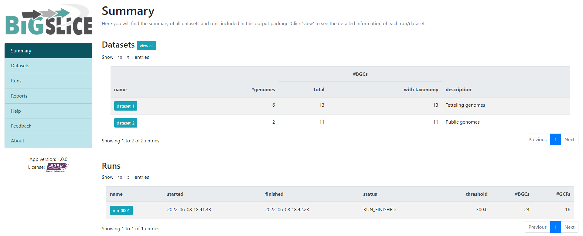
Here we have a summary of the obtained results. In the left part, we
see a set of 7 fields. 3 of them have the information that we generated:
Summary, Datasets, and Runs. The
other ones are for information regarding the software, one of them is to
give feedback to the developers. You can acces to the
Datasets and Runs page also from the options
that we see in the main part of this summary page. The first part of
this summary describes the datasets that we provided as input. The
second one is the information of the process (when we ran the program)
that BiG-SLiCE carry out with our data.
If we click into the Runs field on the left or the
run-0001 blue button on the Runs main
section, we will jump into the page that gives us the information
regarding the BGCs GCFs that were obtained:
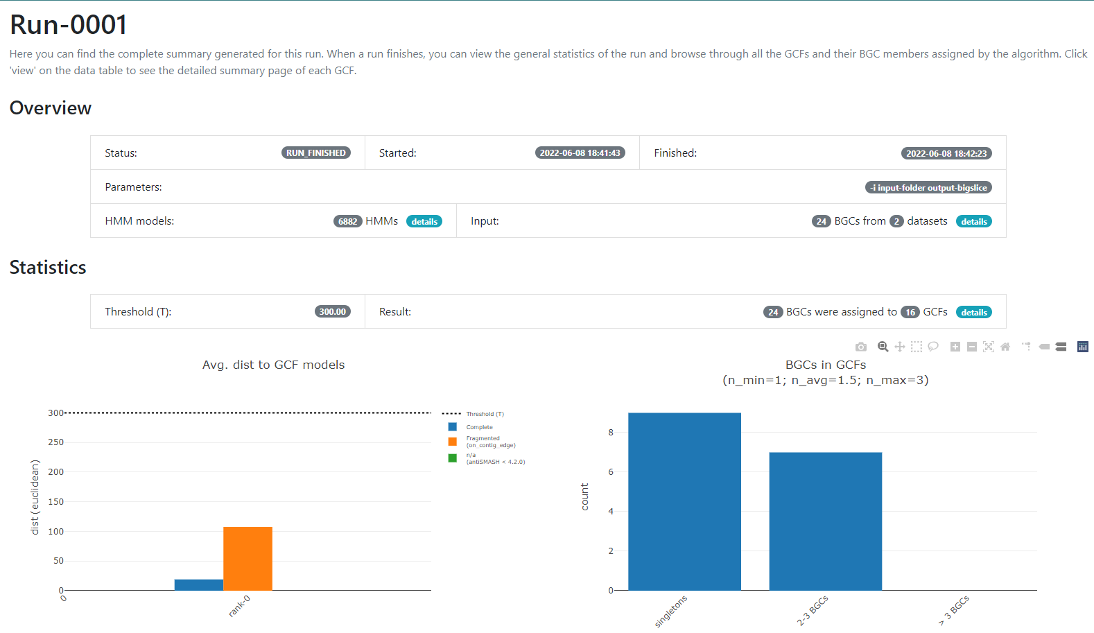
In this new page we have two bar-plots that give us information
regarding if the BGCs that we sumministrated were classified as
fragmented or complete by AntiSMASH (according to the
AntiSMASH algorithm, a BGC can be classified as fragmented
if it is found at the edge of a contig), and how many families were
obtained with singletons (composed of just one BGC) and of 2-3 BGCs.
If we go to the bottom of this page, we will found a table of all the GCFs with information of the number of BGCs that compose them, the representative BGC class inside each family, and which genus has more BGCs that belong to each family.
Click the + symbol of the GCF_7, and then on the
View button that is displayed. This will take us to a page
with statistics of the BGCs that are part of this family.
Inside this section, we can found a great amount of information
regarding the GCF_7 BGC’s. If we jump to section called
Members, we can click on the view BGC arrowers
button to get a visualization of the domains that are part of each of
the genes of these BGCs.
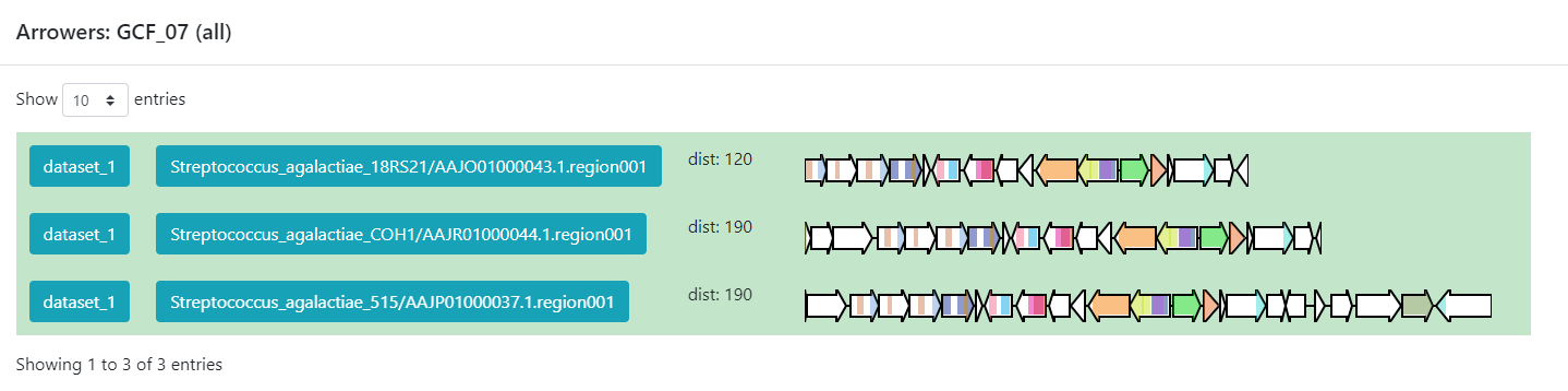
As we can see, this tool can be used to clusterize homologous BGCs that share a structure. With this knowledge, we can try some hypothesis or even build new ones in the light of this information.
Discussion
Considering the results in the runs tab, we can see that there are a
lot of Gene Cluster Families that have only one cluster associated to it
(GCF_1, GCF_2, GCF_4, GCF_5, GCF_6, GCF_8, GCF_9, GCF_13, and GCF_15).
What does this tell us about the metabolites diversity of the
Streptococcus sample?
We can see that there are some unique gene cluster families, which means that there are an organism that has that unique gene cluster and therefore it has some metabolite that the others don´t and that may be advantageous in its environment. Since there are many singleton Gene Cluster Families, we can say that there is a big diversity from the sample because many of the organisms in the sample have unique “abilities” (metabolites).
Discussion
Suppose we get the following results from a sample of 6 organisms.
|——————-+——————————————————–| | GCF | #core members | |:—————–:+:——————————————————:| | GCF_1 | 6 | |——————-+——————————————————–| | GCF_2 | 5 | |——————-+——————————————————–| | GCF_3 | 5 | |——————-+——————————————————–| | GCF_4 | 6 | |——————-+——————————————————–|
What can we infer about the metabolite diversity?
As most of the organisms have a gene cluster in the gene cluster family, we can infer that most of them have the same secondary metabolites, which means that there is little metabolite diversity between them.
BiG-FAM
To demonstrate the functionality of BiG-SLICE, the
authors gathered close to 1.2 million of BGCs. All this information,
they put it on a great database that they called BiG-FAM.
When you get to the main page, you will face a
structure that looks like the one we saw on the BiG-SLICE
results:
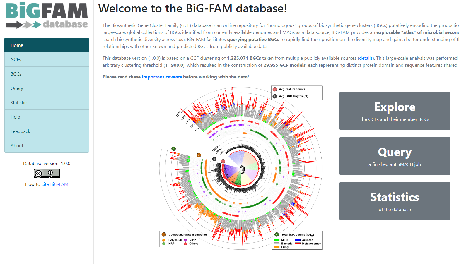
One of the options on the left is Query. If we click
here, we will move to a new page where we can insert an
antiSMASH job ID. This will run a comparison of all the
BGCs found on that antiSMASH run on a single genome, against the immense
database.
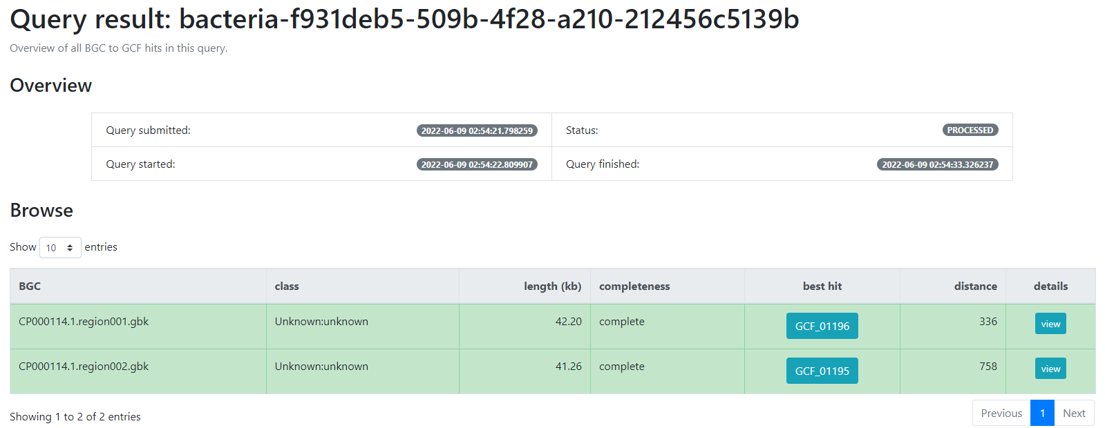
We will use the antiSMASH job ID from the analysis made
on Streptococcus agalactiae A909. The
antiSMASH job ID can be found in the URL
direction of this page in the next format:
taxon-aaaaaaa-bbbb-cccc-dddd-eeeeeeeeeeee.
We will use the job ID that we obtained:
bacteria-f931deb5-509b-4f28-a210-212456c5139b
And click the submit option.
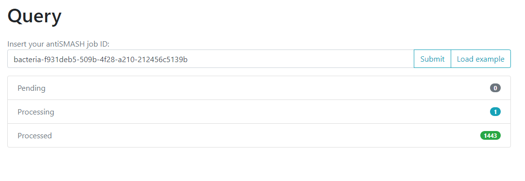
This will generate a result page that indicates with which BGCs from the database, the BGCs from the query genome are related.
-
BiG-SLiCEandBiG-FAMare softwares that are useful to compare the metabolic diversity of bacterial lineages between each other and against a big database - An input-folder containing the BGCs from antiSMASH and the taxonomic
information of each genome is needed to run
BiG-SLiCE - The results from the antiSMASH web-tool are needed to run
BiG-FAM - Gene Cluster Families can help us to compare the metabolic capabilities of a set of bacterial lineages
- We can use
BiG-FAMto compare a BGC against the whole database and predict its Gene Cluster Family