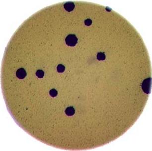
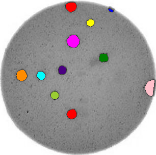
Image 1 of 1: ‘Bacteria colony’
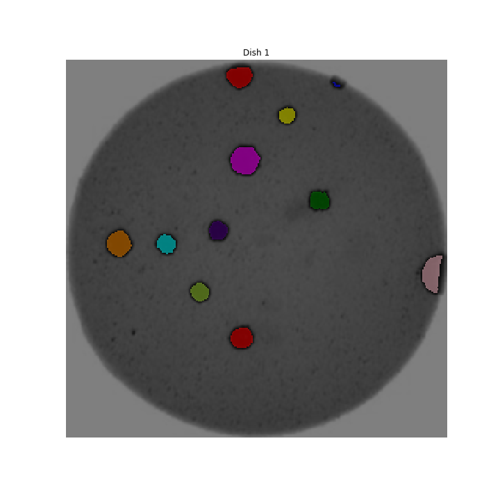
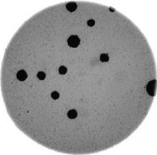
Image 1 of 1: ‘Colonies counted’
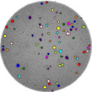
Image 1 of 1: ‘Bacteria colony’
Image 1 of 1: ‘Original size image’
Image 1 of 1: ‘Enlarged image area’
Image 1 of 1: ‘Image of 8’
Image 1 of 1: ‘Image of 0’
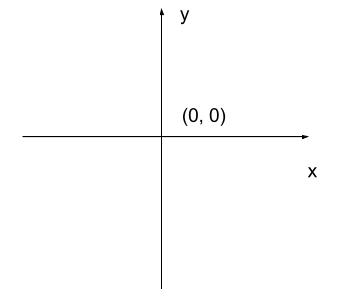
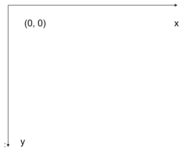
Image 1 of 1: ‘Cartesian coordinate system’
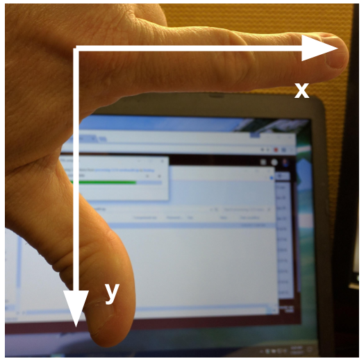
Image 1 of 1: ‘Image coordinate system’
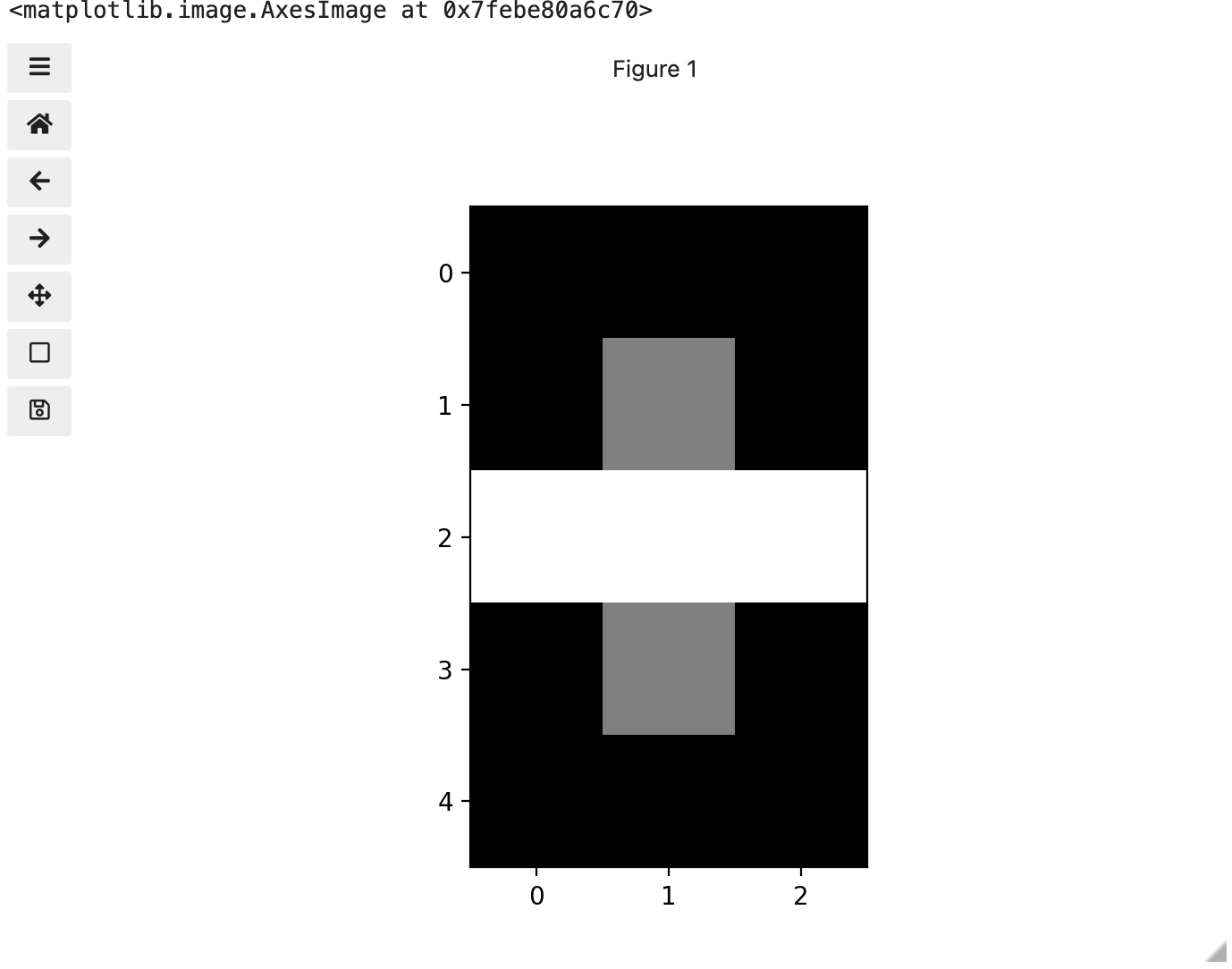
Image 1 of 1: ‘Left-hand coordinate system’
Image 1 of 1: ‘Image of 5’
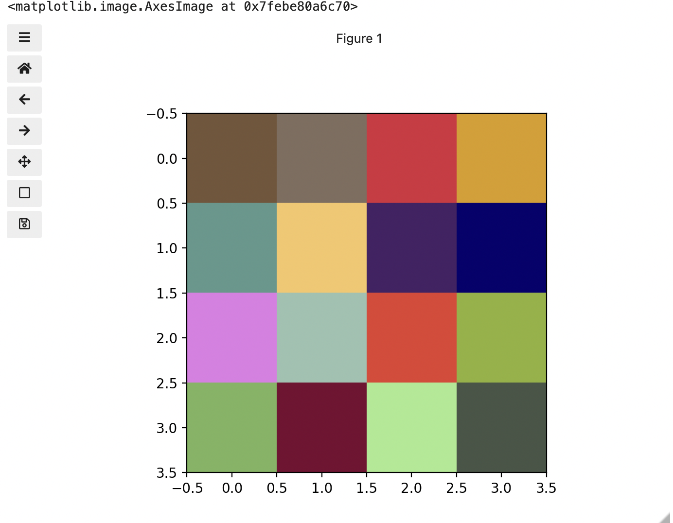
Image 1 of 1: ‘Image of three colours’
Image 1 of 1: ‘Image in greyscale’
Image 1 of 1: ‘Image of checkerboard’
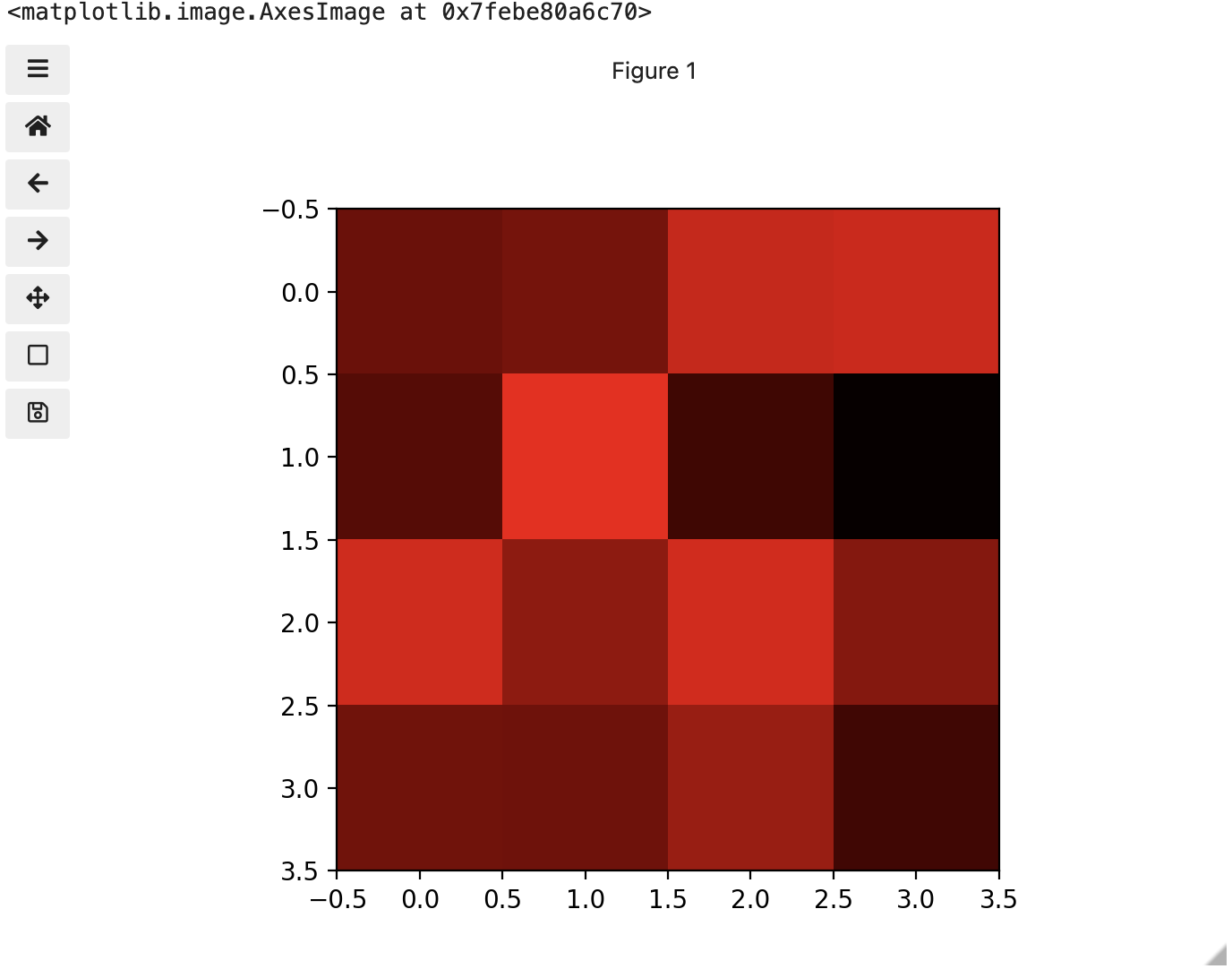
Image 1 of 1: ‘Image of red channel’
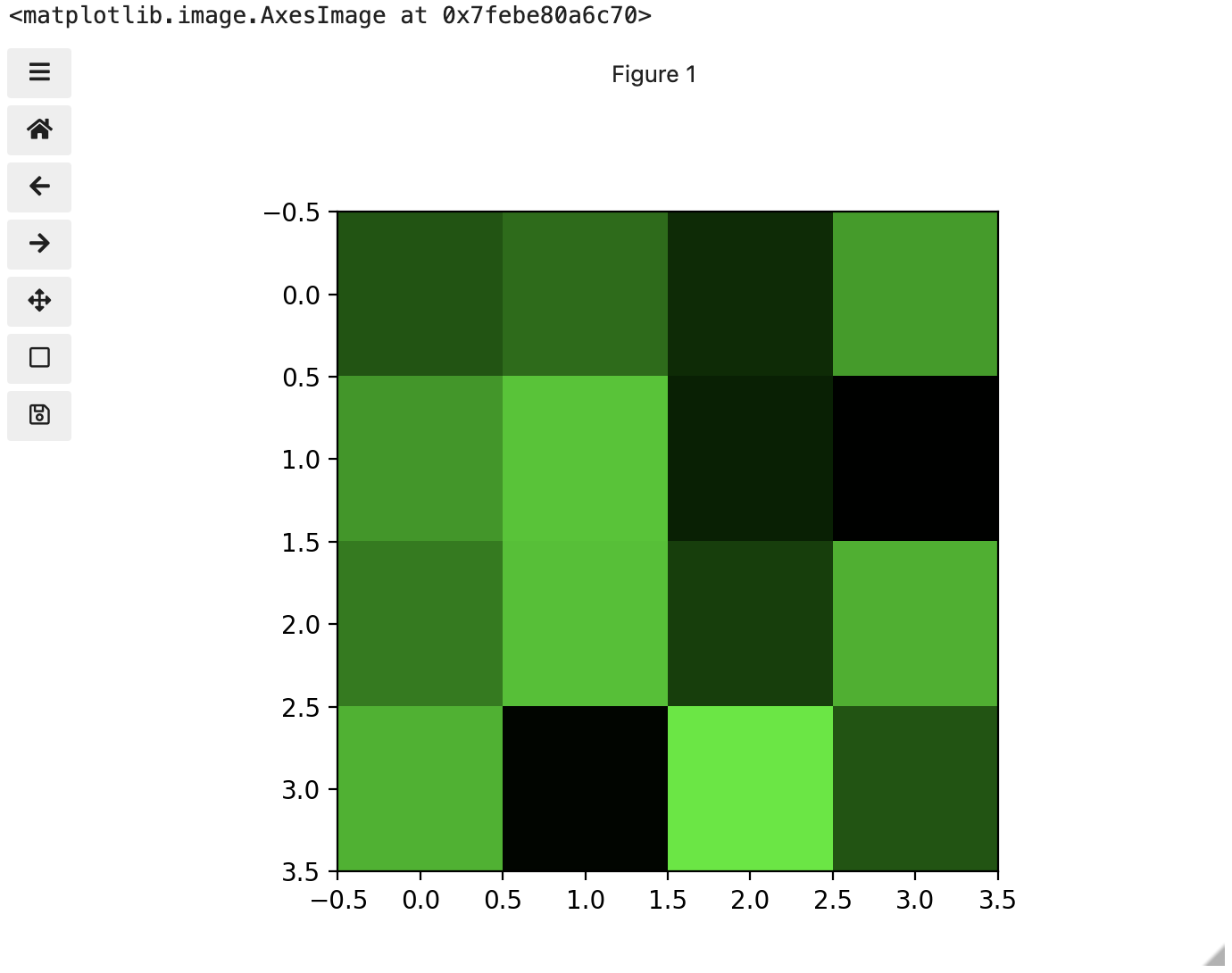
Image 1 of 1: ‘Image of green channel’
Image 1 of 1: ‘Image of blue channel’
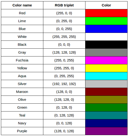
Image 1 of 1: ‘RGB colour table’
Image 1 of 1: ‘Original image’
Image 1 of 1: ‘Enlarged, uncompressed’
Image 1 of 1: ‘Enlarged, compressed’
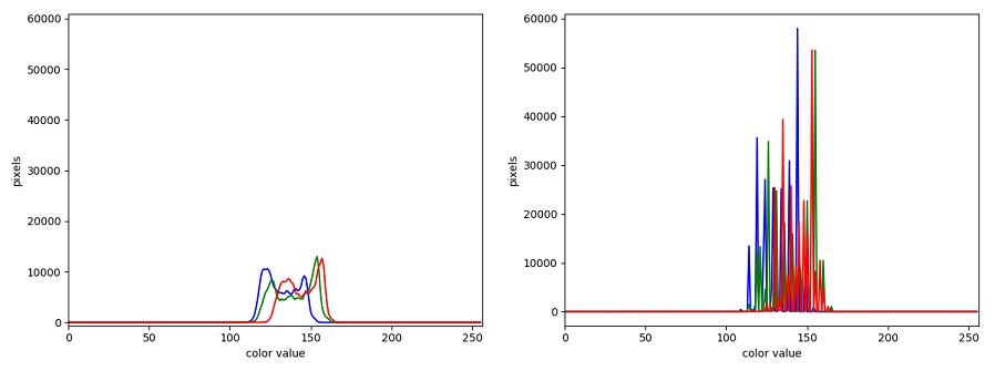
Image 1 of 1: ‘Uncompressed histogram’
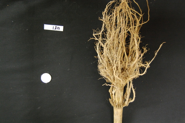
Image 1 of 1: ‘Root cluster image’
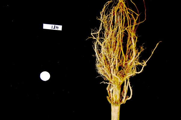
Image 1 of 1: ‘Thresholded root image’
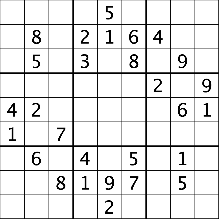
Image 1 of 1: ‘Su-Do-Ku puzzle’
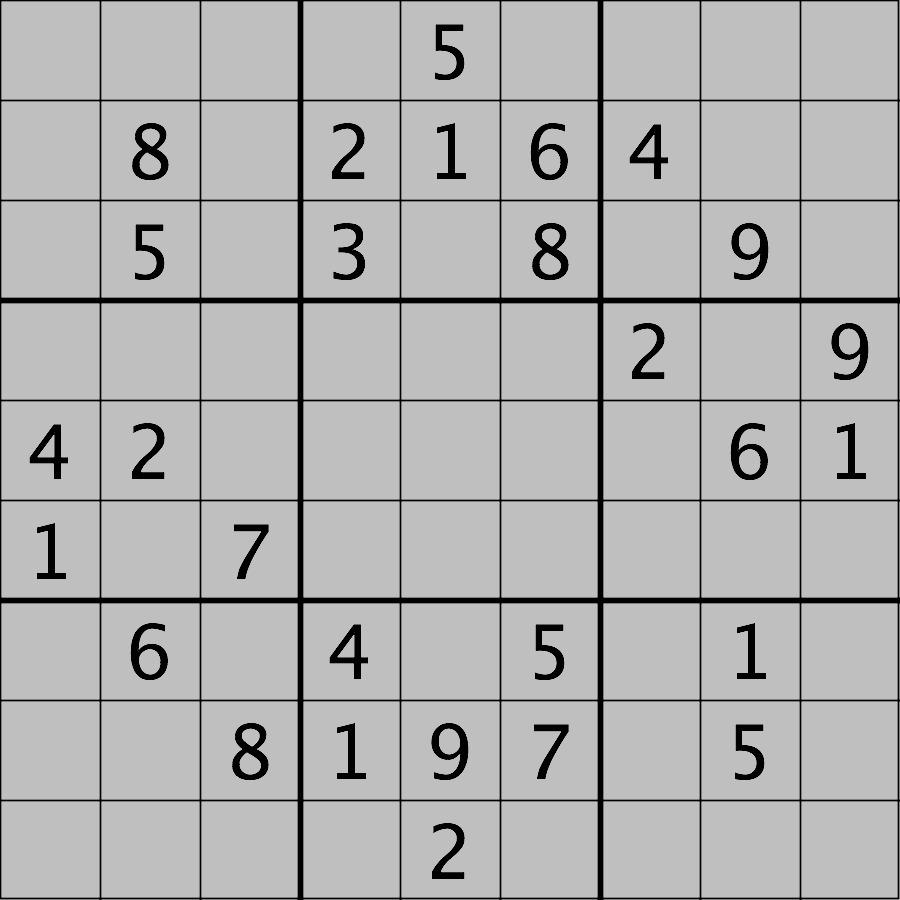
Image 1 of 1: ‘Modified Su-Do-Ku puzzle’
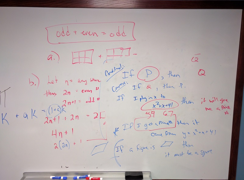
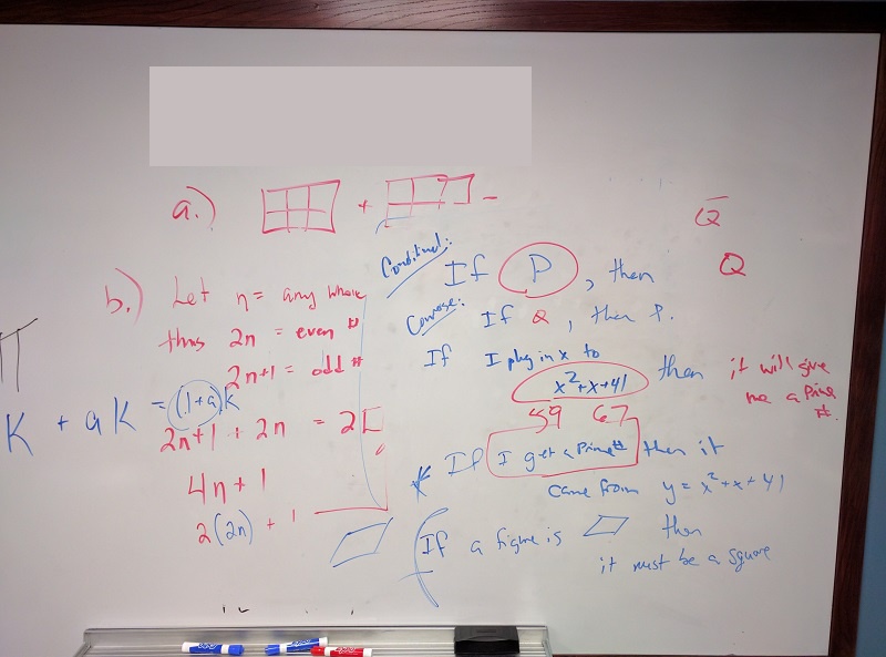
Image 1 of 1: ‘Whiteboard image’
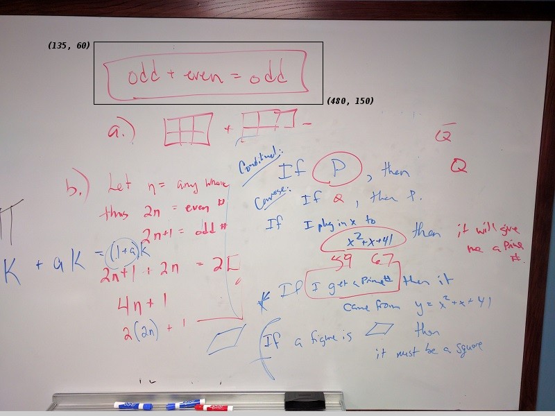
Image 1 of 1: ‘Whiteboard coordinates’
Image 1 of 1: ‘"Erased" whiteboard’
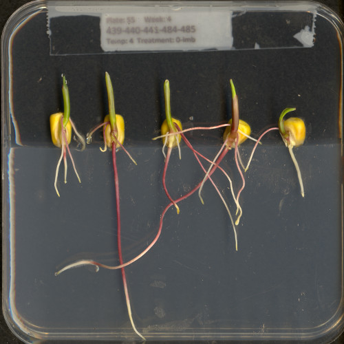
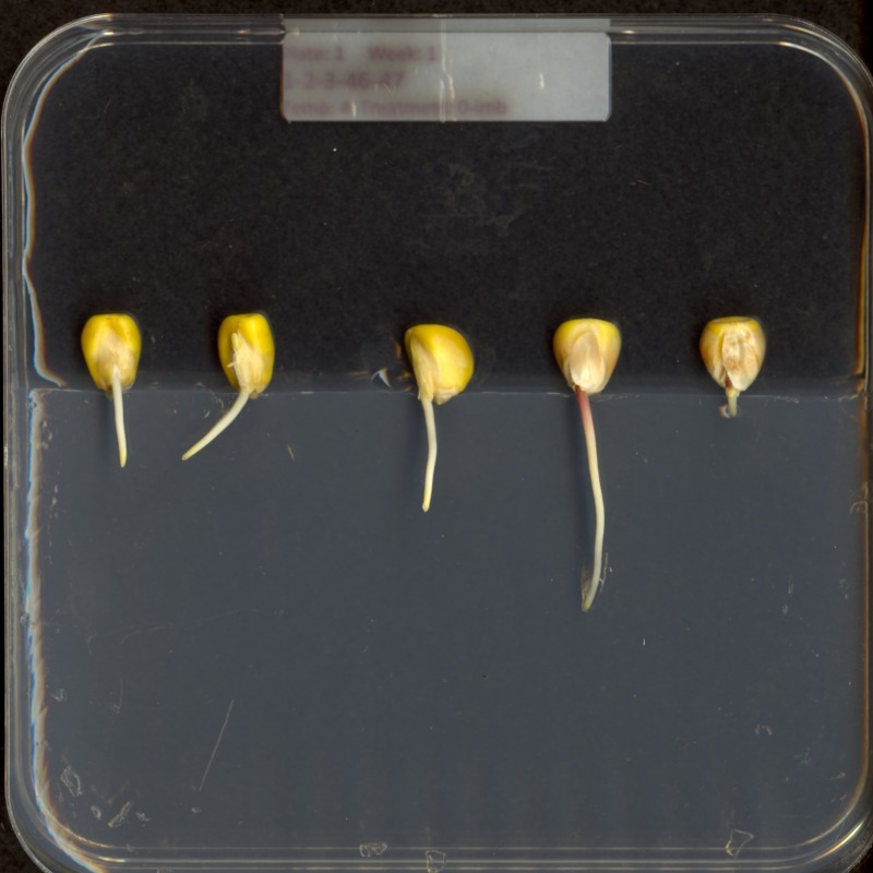
Image 1 of 1: ‘Maize seedlings’
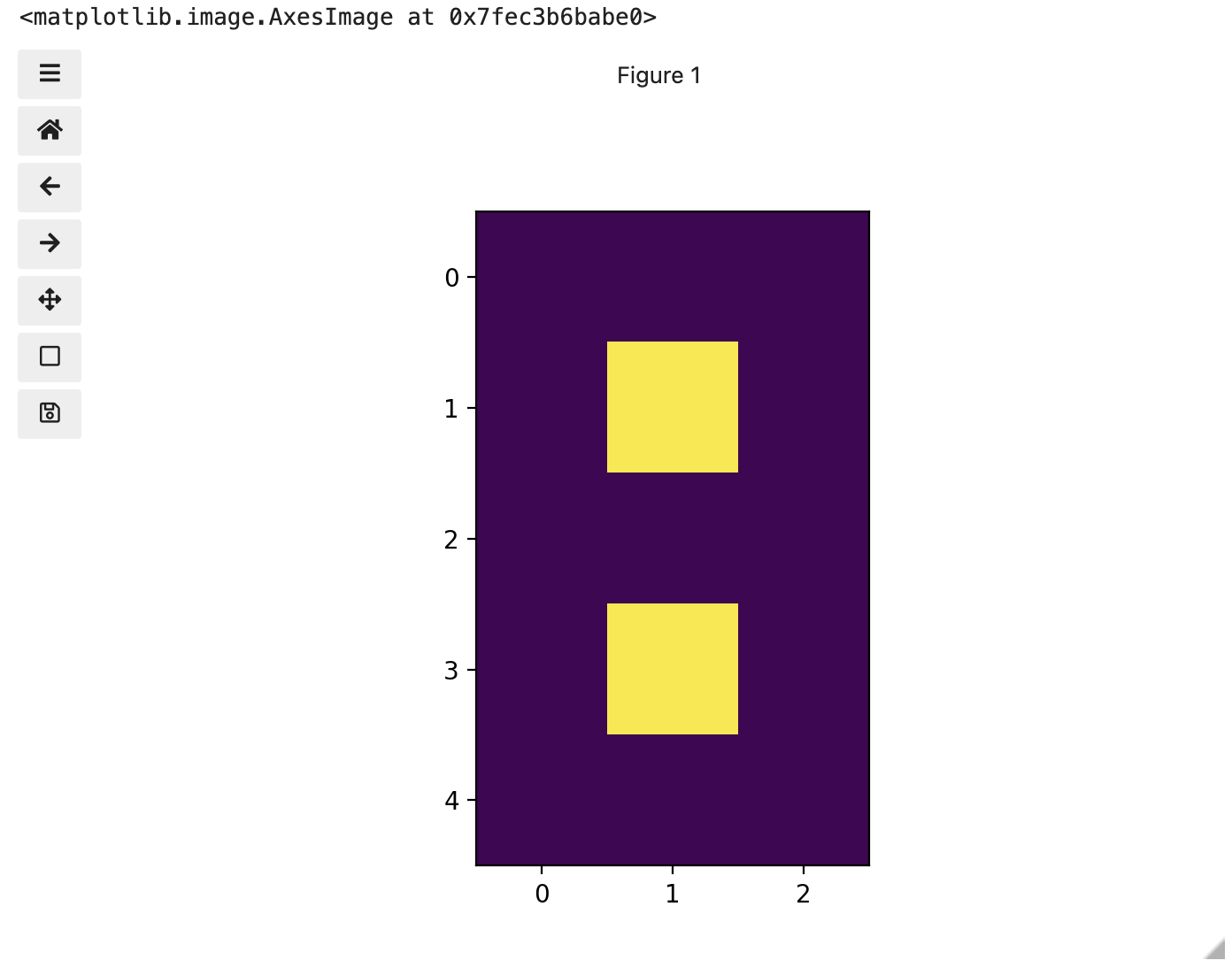
Image 1 of 1: ‘Maize image mask’
Here is what our constructed mask looks like:
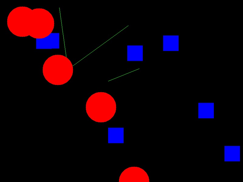
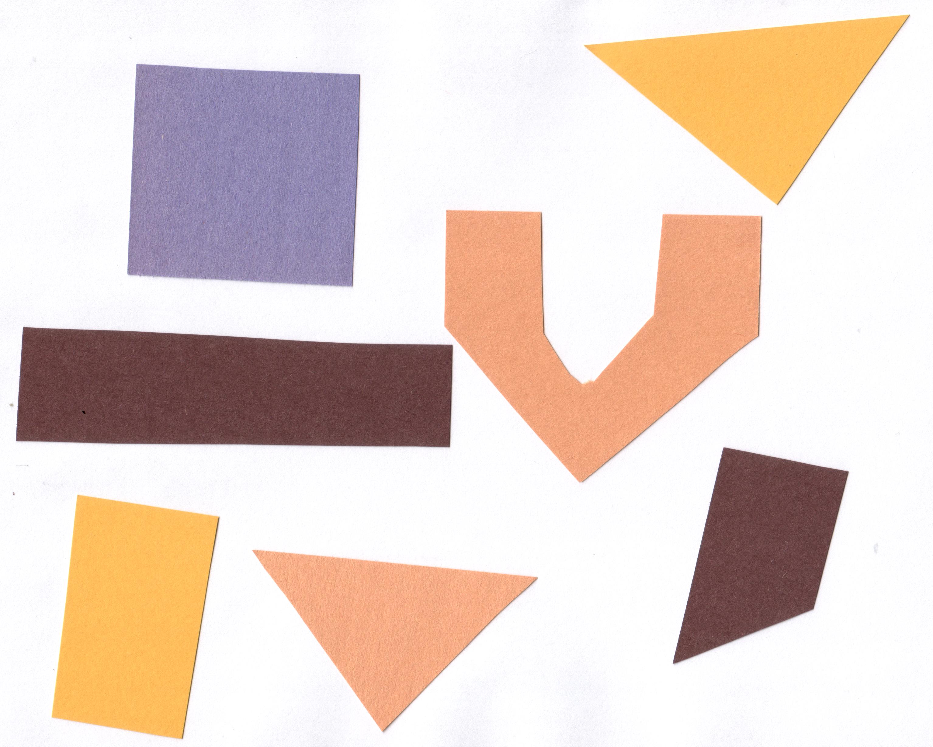
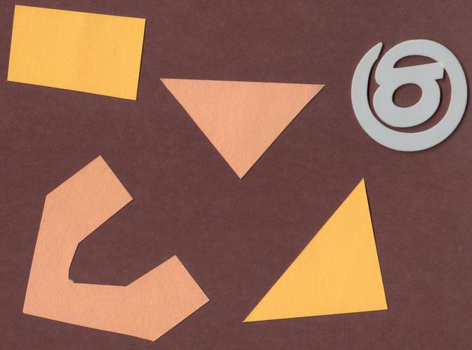
Image 1 of 1: ‘Sample shapes’
Image 1 of 1: ‘Applied mask’
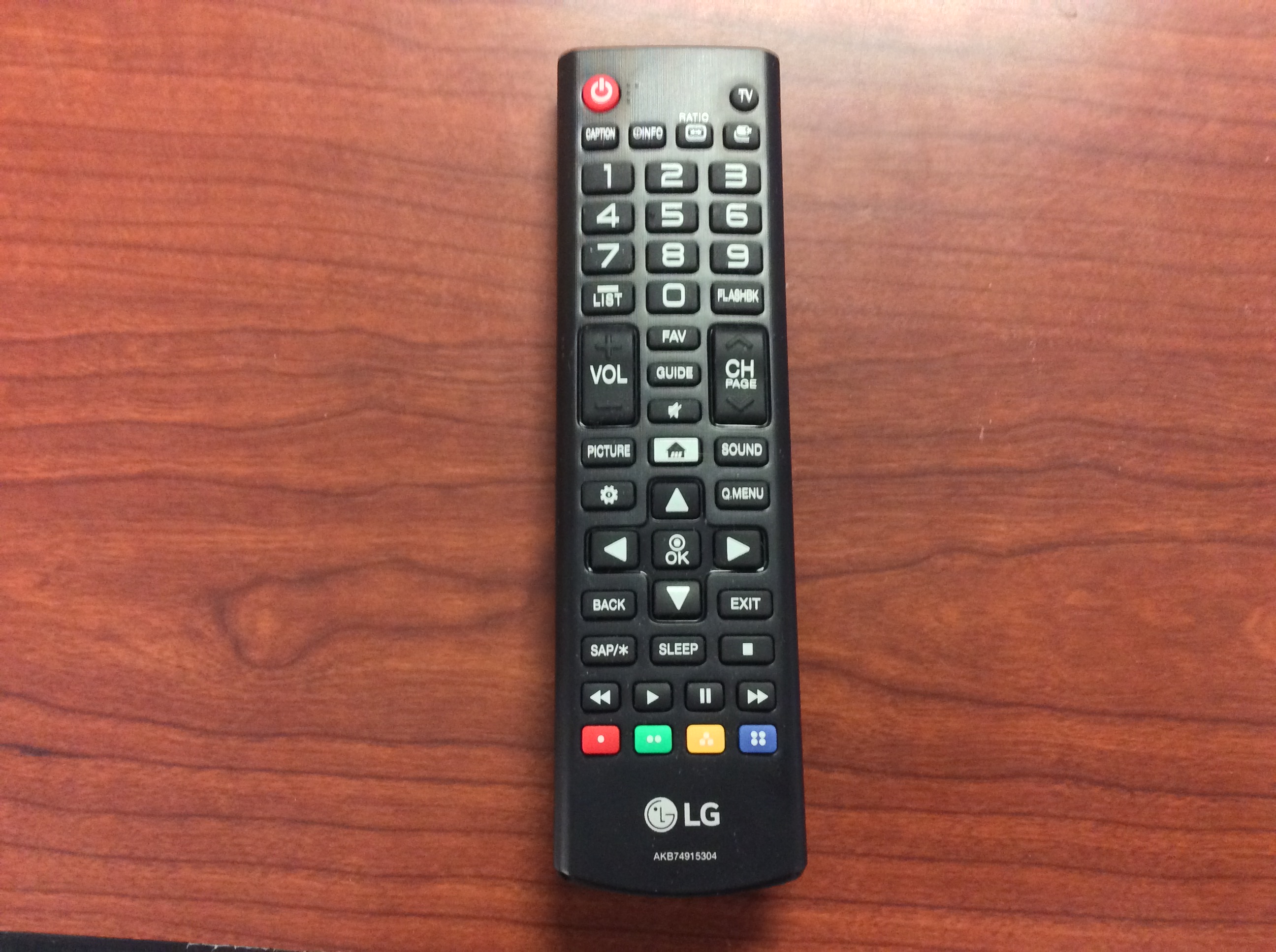
Image 1 of 1: ‘Remote control image’
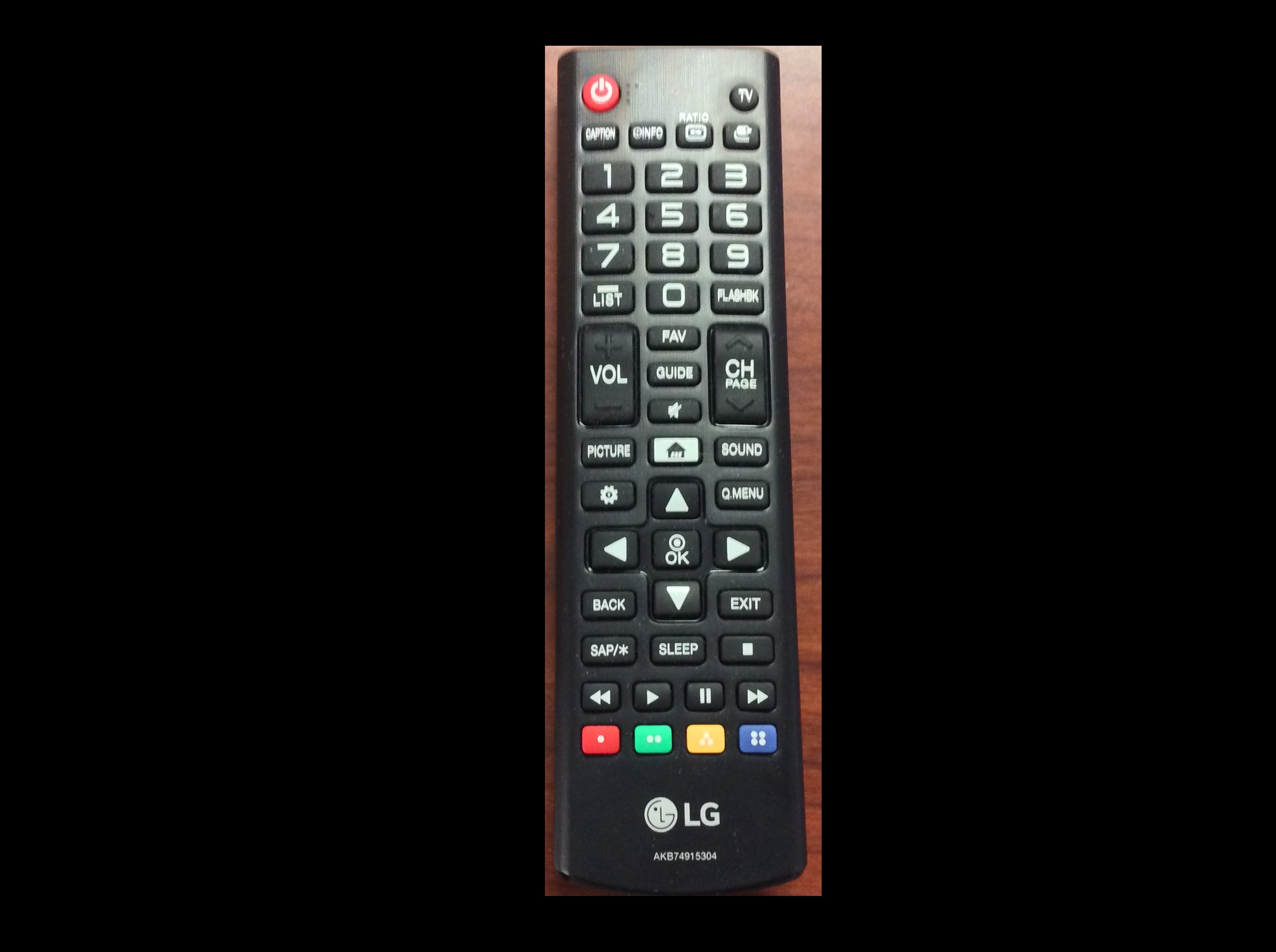
Image 1 of 1: ‘Remote control masked’
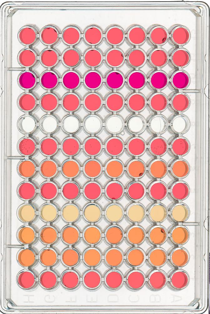
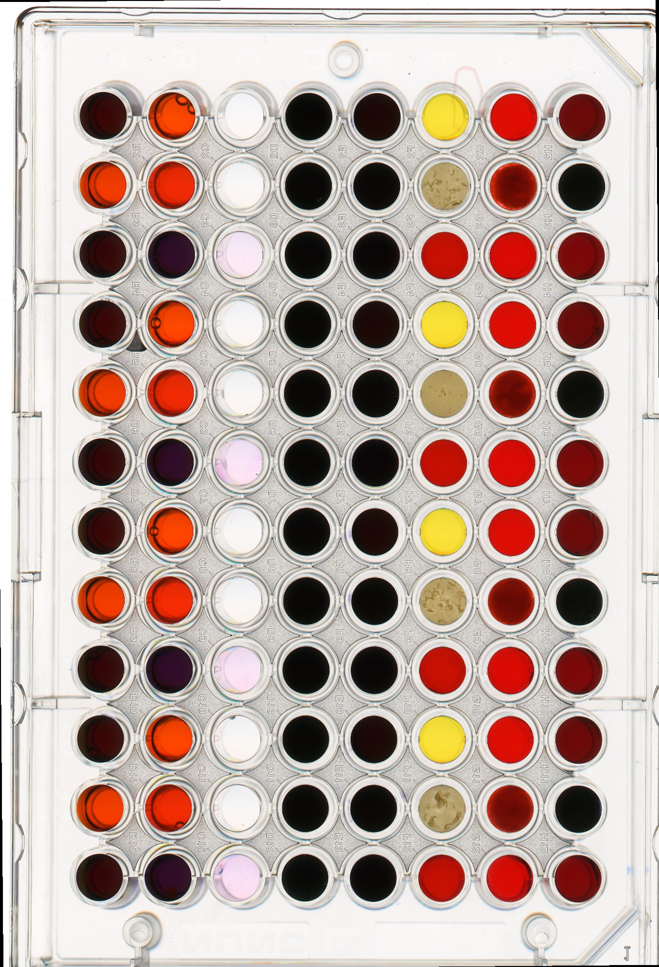
Image 1 of 1: ‘96-well plate’
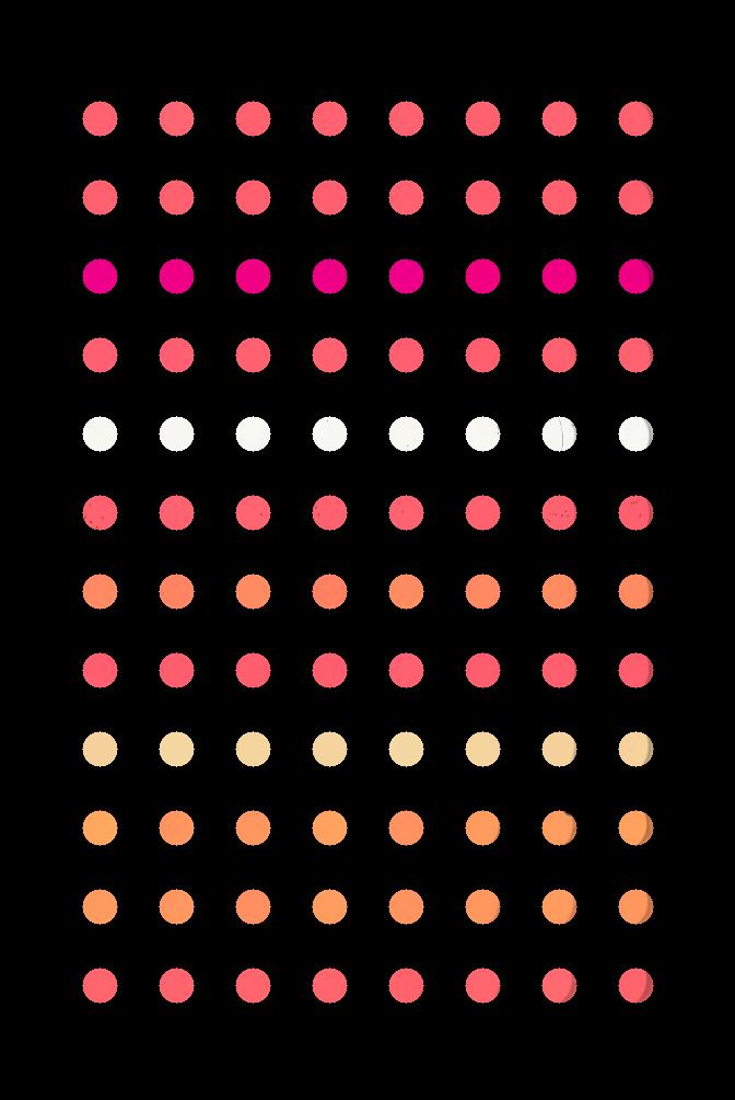
Image 1 of 1: ‘Masked 96-well plate’
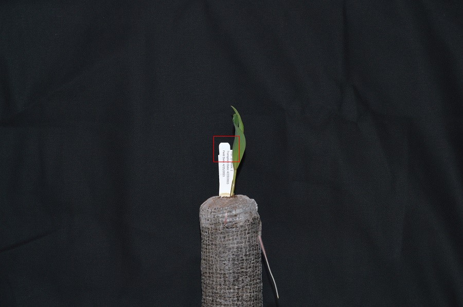
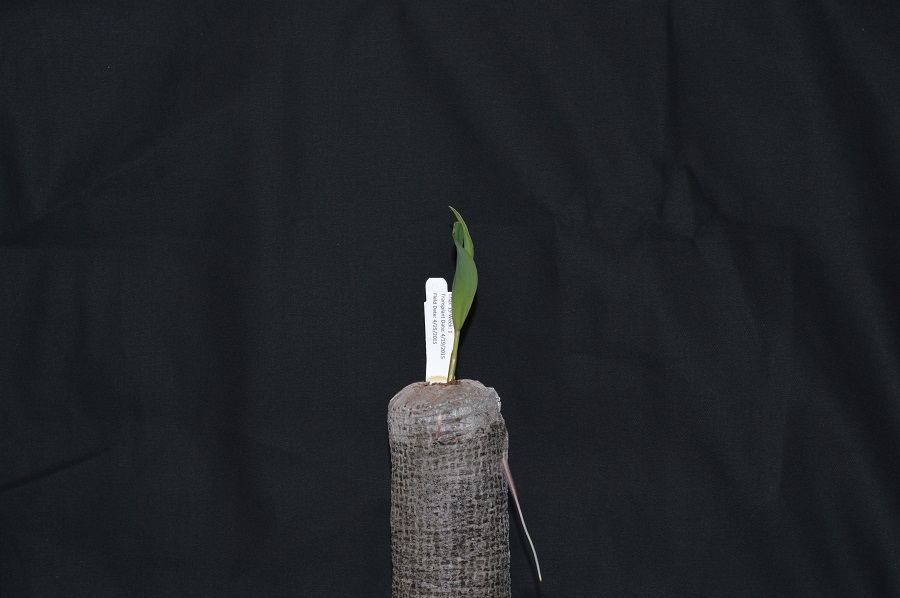
Image 1 of 1: ‘Plant seedling’
We will start with grayscale images, and then move on to colour
images. We will use this image of a plant seedling as an example:
Image 1 of 1: ‘Plant seedling’
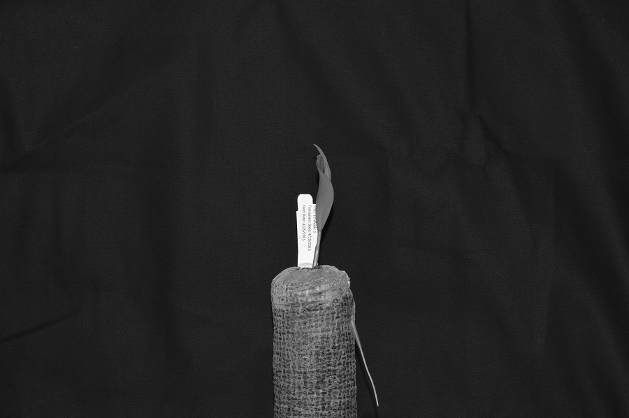
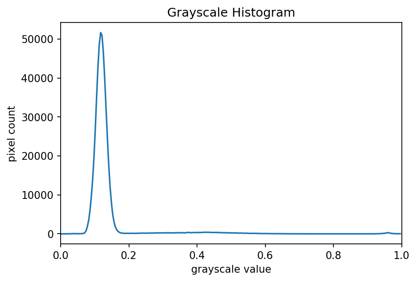
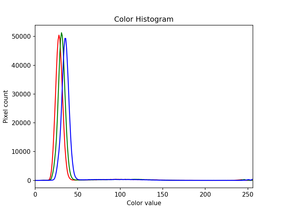
Image 1 of 1: ‘Plant seedling histogram’
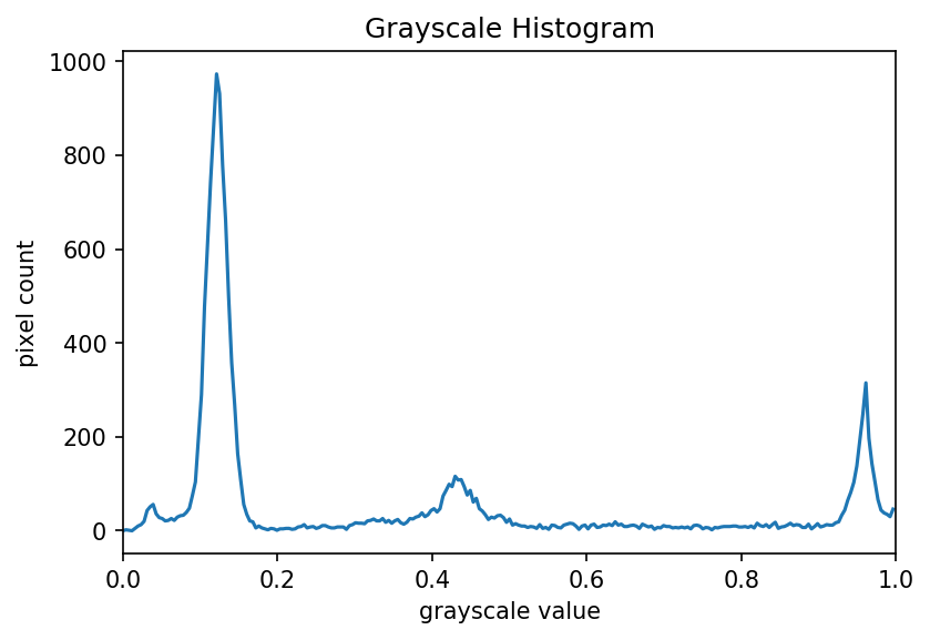
Image 1 of 1: ‘Grayscale histogram of masked area’
Image 1 of 1: ‘Colour histogram’
Image 1 of 1: ‘Well plate image’
Image 1 of 1: ‘Masked well plate’
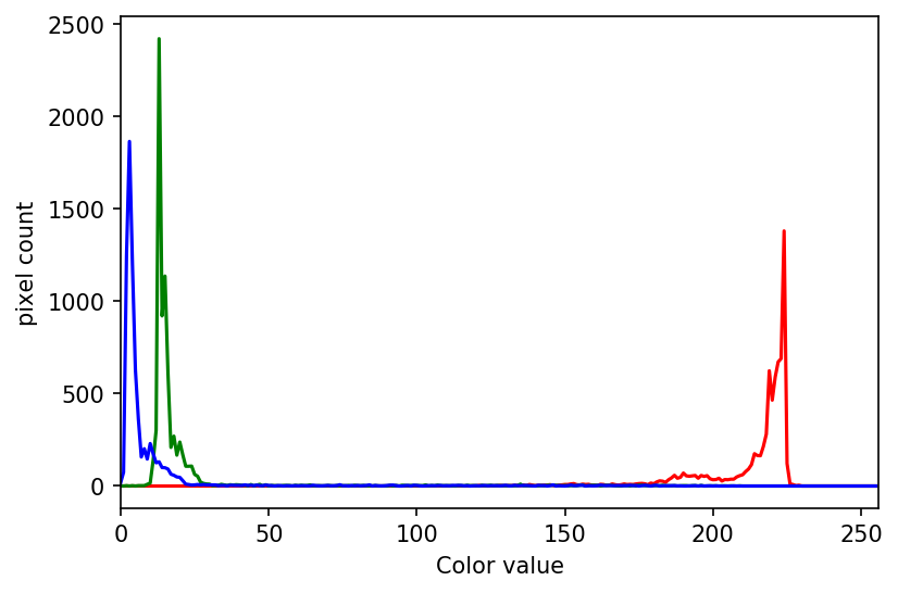
Image 1 of 1: ‘Well plate histogram’
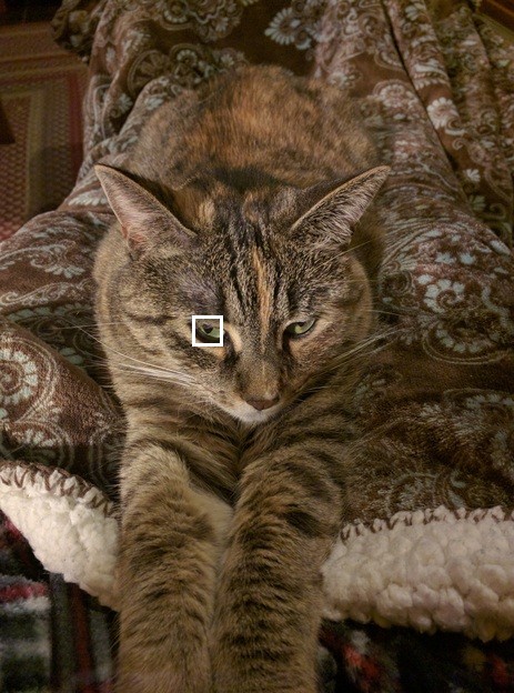
Image 1 of 1: ‘Cat image’
Image 1 of 1: ‘Cat eye pixels’
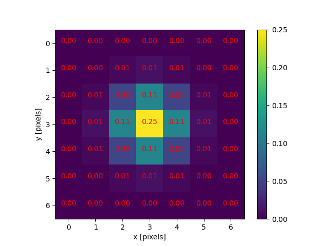
Image 1 of 1: ‘Gaussian function’
A Gaussian function maps random variables into a normal distribution
or “Bell Curve”.
Image 1 of 1: ‘2D Gaussian function’
Image 1 of 1: ‘2D Gaussian function’
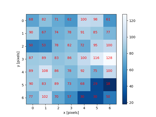
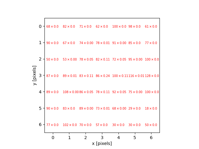
Image 1 of 1: ‘Image corner pixels’
Image 1 of 1: ‘Image multiplication’
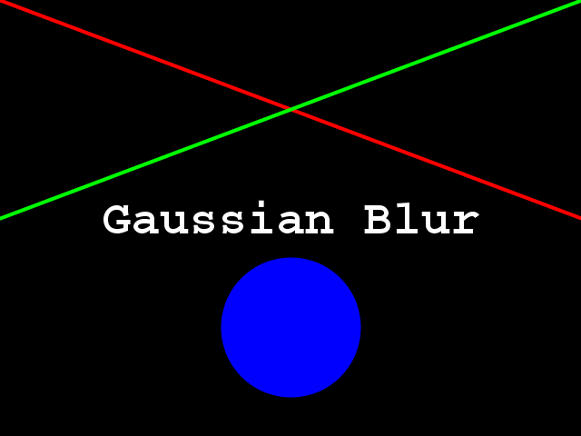
Image 1 of 1: ‘Blur demo animation’
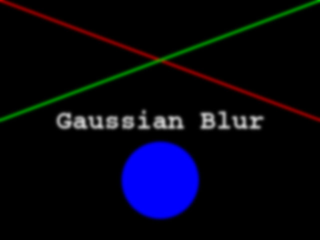
Image 1 of 1: ‘Original image’
Image 1 of 1: ‘Blurred image’
Image 1 of 1: ‘Bacteria colony’
Graysacle version of the Petri dish image
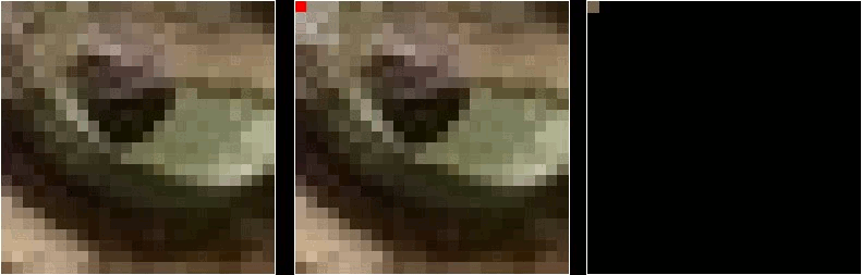
Image 1 of 1: ‘Bacteria colony image with selected pixels marker’
Grayscale Petri dish image marking selected
pixels for profiling
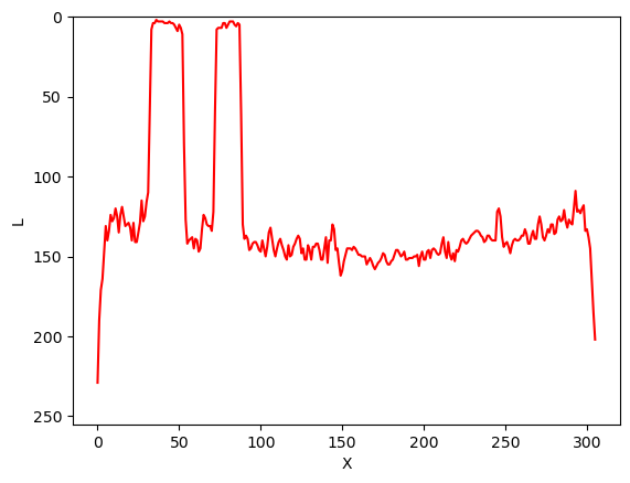
Image 1 of 1: ‘Pixel intensities profile in original image’
Intensities profile line plot of pixels along
Y=150 in original image
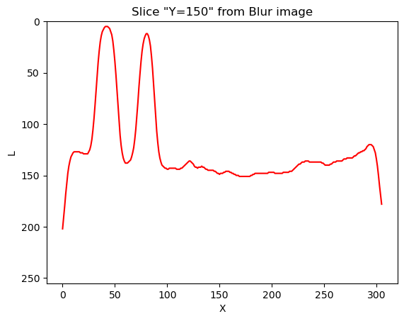
Image 1 of 1: ‘Pixel intensities profile in blurred image’
Intensities profile of pixels along Y=150 in
blurred image
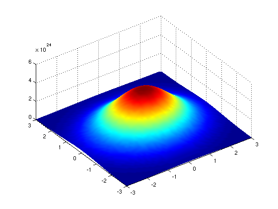
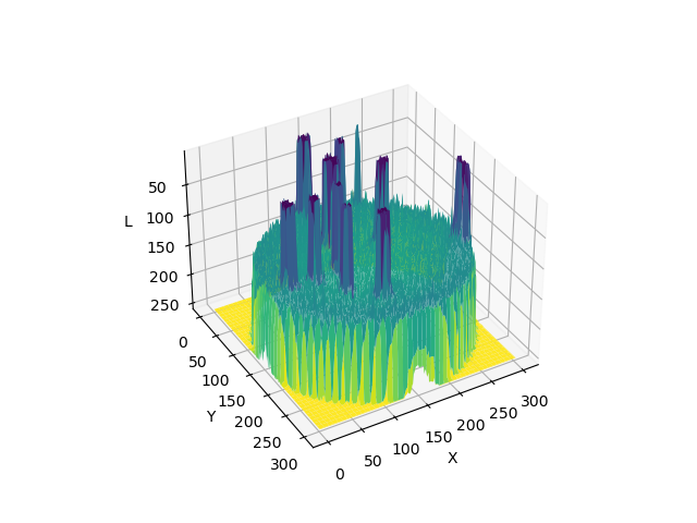
Image 1 of 1: ‘3D surface plot showing pixel intensities across the whole example Petri dish image before blurring’
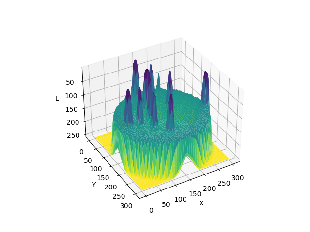
Image 1 of 1: ‘3D surface plot illustrating the smoothing effect on pixel intensities across the whole example Petri dish image after blurring’
A 3D plot of pixel intensities after Gaussian
blurring of the Petri dish image. Note the ‘smoothing’ effect on the
pixel intensities of the colonies in the image, and the ‘flattening’ of
the background noise at relatively low pixel intensities throughout the
image.
Explore
how this plot was created with matplotlib . Image credit:
Carlos H Brandt .
Image 1 of 1: ‘Rectangular kernel blurred image’
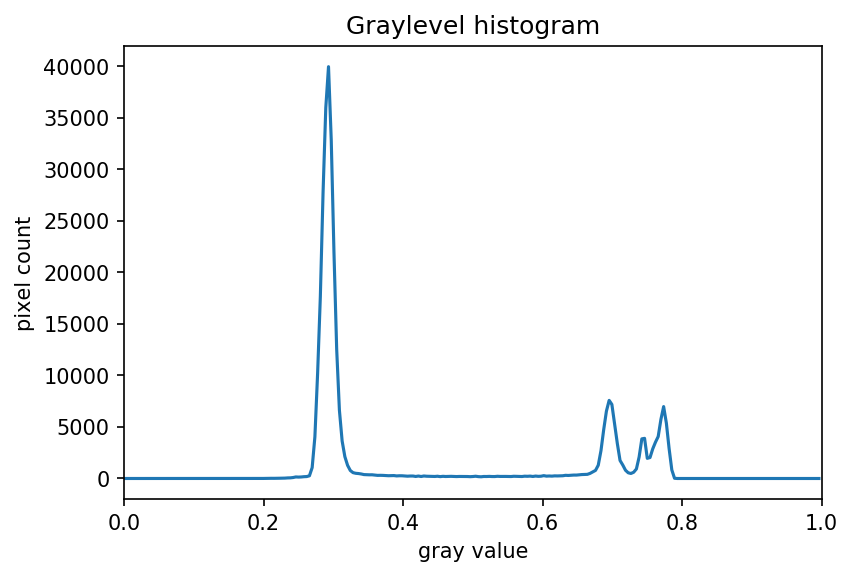
Image 1 of 1: ‘Image with geometric shapes on white background’
Image 1 of 1: ‘Grayscale image of the geometric shapes’
Image 1 of 1: ‘Grayscale histogram of the geometric shapes image’
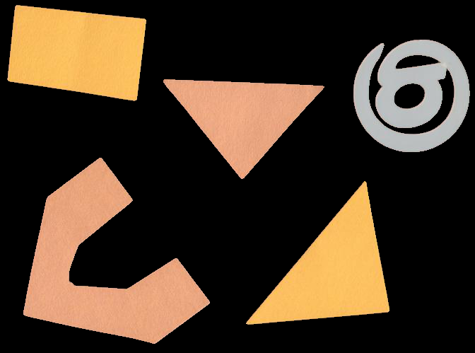
Image 1 of 1: ‘Binary mask of the geometric shapes created by thresholding’
Image 1 of 1: ‘Selected shapes after applying binary mask’
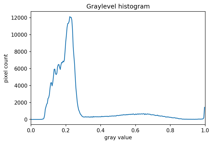
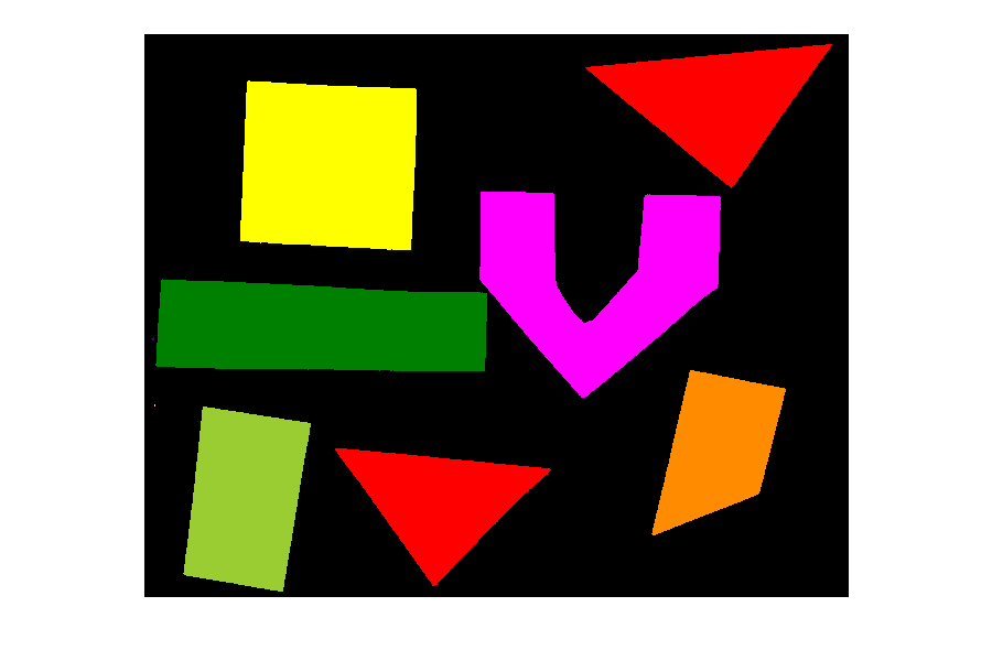
Image 1 of 1: ‘Another image with geometric shapes on white background’
Image 1 of 1: ‘Grayscale histogram of the second geometric shapes image’
Image 1 of 1: ‘Binary mask created by thresholding the second geometric shapes image’
Image 1 of 1: ‘Selected shapes after applying binary mask to the second geometric shapes image’
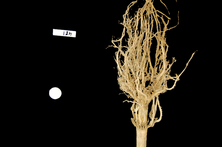
Image 1 of 1: ‘Image of a maize root’
Image 1 of 1: ‘Grayscale histogram of the maize root image’
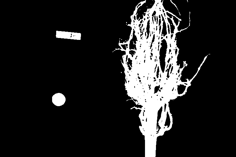
Image 1 of 1: ‘Binary mask of the maize root system’
Image 1 of 1: ‘Masked selection of the maize root system’
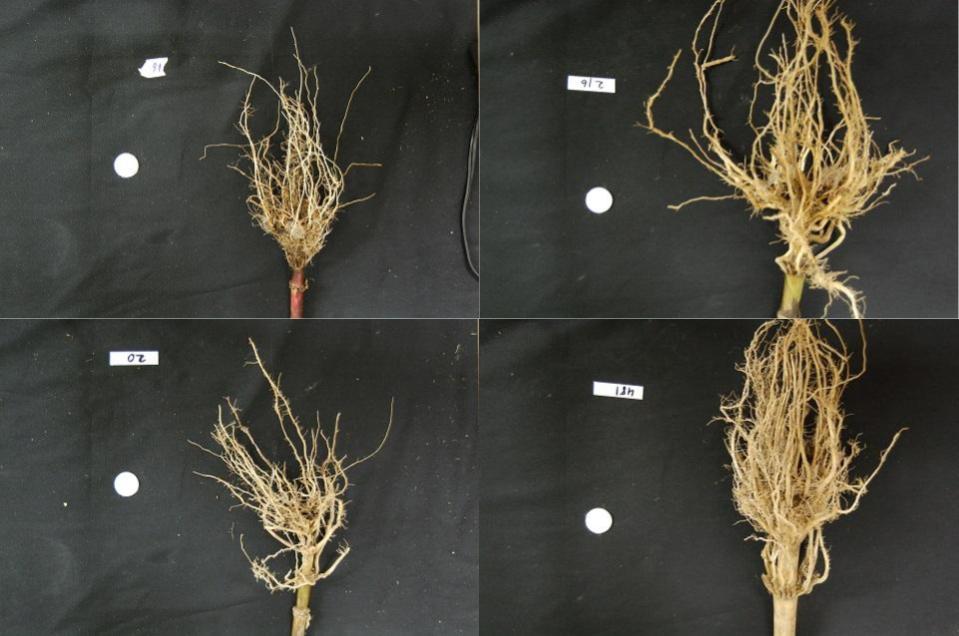
Image 1 of 1: ‘Four images of maize roots’
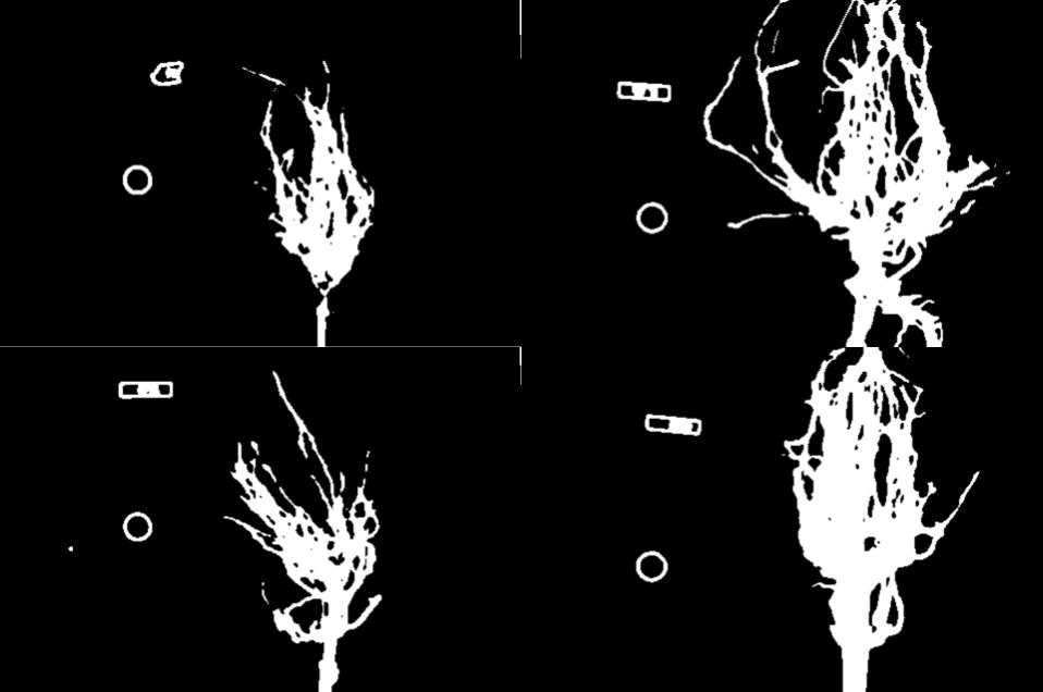
Image 1 of 1: ‘Binary masks of the four maize root images’
Image 1 of 1: ‘Improved binary masks of the four maize root images’
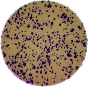
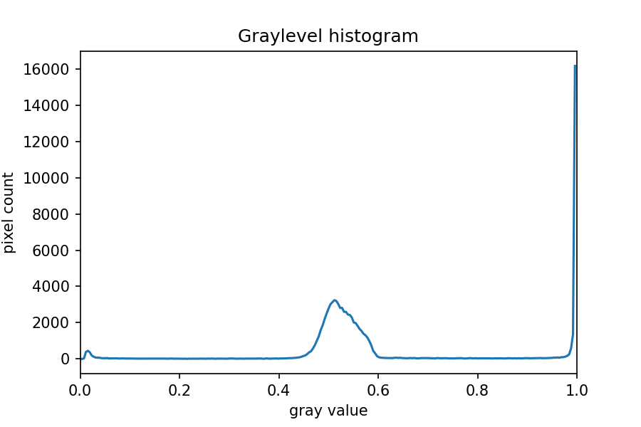
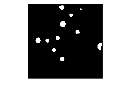
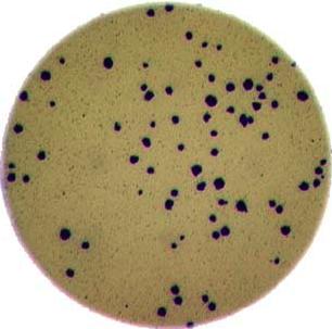
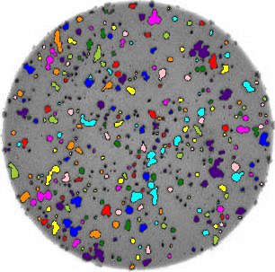
Image 1 of 1: ‘Image of bacteria colonies in a petri dish’
Image 1 of 1: ‘Grayscale histogram of the bacteria colonies image’
Image 1 of 1: ‘Binary mask of the bacteria colonies image’
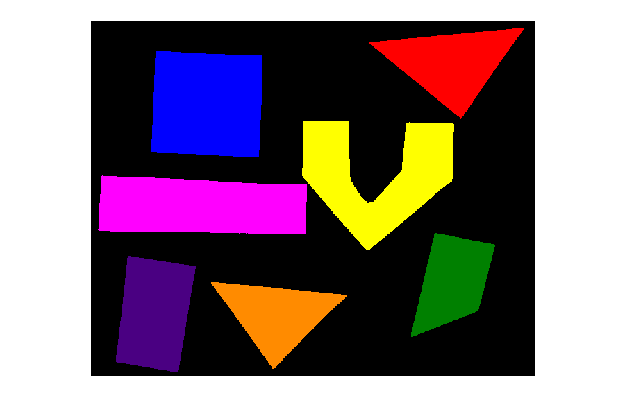
Image 1 of 1: ‘Original shapes image’
Image 1 of 1: ‘Mask created by thresholding’
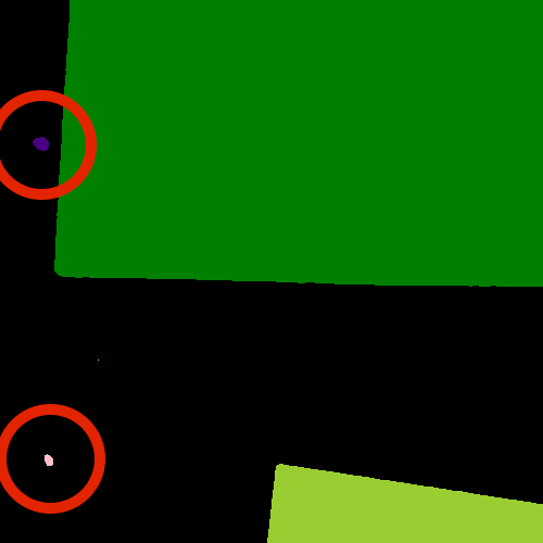
Image 1 of 1: ‘Labeled objects’
Image 1 of 1: ‘shapes-01.jpg mask detail’
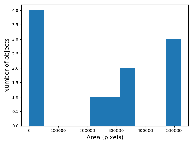
Image 1 of 1: ‘Histogram of object areas’
Image 1 of 1: ‘Objects filtered by area’
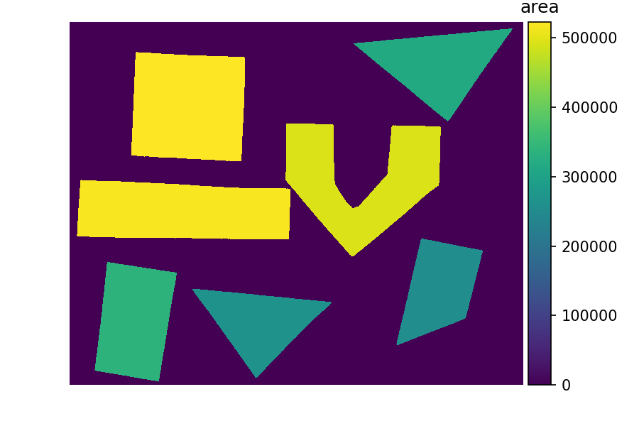
Image 1 of 1: ‘Objects colored by area’
Image 1 of 1: ‘Colony image 1’
Image 1 of 1: ‘Colony image 2’
Image 1 of 1: ‘Colony image 3’
Image 1 of 1: ‘Sample morphometric output’
Image 1 of 1: ‘Colony image 1’
Image 1 of 1: ‘Gray Colonies’
Image 1 of 1: ‘Histogram image’
Image 1 of 1: ‘Colony mask image’
Image 1 of 1: ‘Sample morphometric output’
Image 1 of 3: ‘Colony 1 output’
Image 2 of 3: ‘Colony 2 output’
Image 3 of 3: ‘Colony 3 output’